Complete Numerical Methods Course

April 20, 2025

Numerical Methods Course - ICTTechTitans

ICTTechTitans

Welcome to the Numerical Methods Course

This site provides a comprehensive guide to Numerical Methods, including detailed notes, formulas, exercises, quizzes, and model/practice sets for exam preparation. Use the navigation bar to explore different sections, and click the "Page Marker" button to quickly jump to specific units and their topics.

Unit 1: Nonlinear Equations
- Bisection Method
- Newton-Raphson Method
Unit 2: Interpolation
- Lagrange Interpolation
Unit 3: Differentiation & Integration
Unit 4: Linear Equations
Unit 5: ODEs
Unit 6: PDEs
Model Set Questions
Practice Set 1
Practice Set 2
Practice Set 3
Practice Set 4
Practice Set 5

Complete Numerical Methods Course

Published on April 19, 2025

Unit 1: Solution of Nonlinear Equations

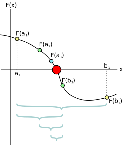
Bisection Method

A method that repeatedly bisects an interval and selects a subinterval where a root exists.

Newton-Raphson Method

Uses the derivative to iteratively approximate roots of a function.

Secant Method

A derivative-free method that uses two initial guesses to approximate roots.

Regula Falsi Method

A method that combines ideas from Bisection and Secant methods to find roots.

Fixed-Point Iteration Method

Rewrites the equation into a fixed-point form and iterates to find the root.

Formulas

Bisection Method: \( c = \frac{a + b}{2} \)IMP

Error in Bisection Method: After \( n \) iterations, the error is at most \( \frac{b - a}{2^n} \).

Newton-Raphson Method: \( x_{n+1} = x_n - \frac{f(x_n)}{f'(x_n)} \)IMP

Secant Method: \( x_{n+1} = x_n - f(x_n) \frac{x_n - x_{n-1}}{f(x_n) - f(x_{n-1})} \)IMP

Regula Falsi Method: \( c = \frac{a f(b) - b f(a)}{f(b) - f(a)} \)IMP

Fixed-Point Iteration: \( x_{n+1} = g(x_n) \)

Convergence Condition for Fixed-Point: \( |g'(x)| < 1 \) near the root.

Exercises (Unit 1)

Find the root of \( x^3 - x - 2 = 0 \) using the Bisection Method in the interval \([1, 2]\) with precision 0.01. [Unit 1, 2078, 10 Marks]

Given \( f(x) = x^3 - x - 2 \), interval \([1, 2]\). Compute: \( f(1) = 1 - 1 - 2 = -2 \), \( f(2) = 8 - 2 - 2 = 4 \). Since \( f(1) \cdot f(2) < 0 \), a root exists. Midpoint \( c = \frac{1 + 2}{2} = 1.5 \), \( f(1.5) = 1.5^3 - 1.5 - 2 = 3.375 - 1.5 - 2 = -0.125 \). New interval \([1.5, 2]\). Next midpoint \( c = 1.75 \), \( f(1.75) \approx 1.359 \). New interval \([1.5, 1.75]\). Continue until precision is met. Final root: \( x \approx 1.521 \).
Solve \( x^2 - 4x - 10 = 0 \) using the Bisection Method in \([5, 6]\). [Unit 1, 2077, 10 Marks]

Given \( f(x) = x^2 - 4x - 10 \), interval \([5, 6]\). Compute: \( f(5) = 25 - 20 - 10 = -5 \), \( f(6) = 36 - 24 - 10 = 2 \). Midpoint \( c = 5.5 \), \( f(5.5) = 30.25 - 22 - 10 = -1.75 \). New interval \([5.5, 6]\). Next midpoint \( c = 5.75 \), \( f(5.75) \approx 0.0625 \). New interval \([5.5, 5.75]\). After iterations, root \( x \approx 5.742 \).
Use the Newton-Raphson Method to find a root of \( x^3 - 5x + 1 = 0 \) starting with \( x_0 = 2 \). [Unit 1, 2076, 10 Marks]

Given \( f(x) = x^3 - 5x + 1 \), \( f'(x) = 3x^2 - 5 \). Start with \( x_0 = 2 \). Compute: \( f(2) = 8 - 10 + 1 = -1 \), \( f'(2) = 12 - 5 = 7 \). Then \( x_1 = 2 - \frac{-1}{7} = 2.1429 \). Next, \( f(2.1429) \approx 0.0616 \), \( f'(2.1429) \approx 8.734 \), so \( x_2 = 2.1429 - \frac{0.0616}{8.734} \approx 2.1358 \). Root \( x \approx 2.136 \).
Solve \( e^x - 3x = 0 \) using the Newton-Raphson Method with \( x_0 = 1 \). [Unit 1, 2075, 10 Marks]

Given \( f(x) = e^x - 3x \), \( f'(x) = e^x - 3 \). Start with \( x_0 = 1 \). Compute: \( f(1) = e - 3 \approx -0.282 \), \( f'(1) = e - 3 \approx -0.282 \). Then \( x_1 = 1 - \frac{-0.282}{-0.282} = 0 \). Next, \( f(0) = 1 \), \( f'(0) = -2 \), so \( x_2 = 0 - \frac{1}{-2} = 0.5 \). After iterations, root \( x \approx 0.619 \).
Find a root of \( x^2 - 3 = 0 \) using the Secant Method with initial guesses \( x_0 = 1 \), \( x_1 = 2 \). [Unit 1, 2074, 10 Marks]

Given \( f(x) = x^2 - 3 \), \( x_0 = 1 \), \( x_1 = 2 \). Compute: \( f(1) = -2 \), \( f(2) = 1 \). Then \( x_2 = 2 - 1 \frac{2 - 1}{1 - (-2)} = 1.6667 \). Next, \( f(1.6667) \approx -0.222 \), so \( x_3 = 1.6667 - (-0.222) \frac{1.6667 - 1}{(-0.222) - (-2)} \approx 1.732 \). Root \( x \approx \sqrt{3} \approx 1.732 \).
Use the Secant Method to solve \( \sin(x) - x/2 = 0 \) with \( x_0 = 1 \), \( x_1 = 2 \). [Unit 1, 2073, 10 Marks]

Given \( f(x) = \sin(x) - x/2 \), \( x_0 = 1 \), \( x_1 = 2 \). Compute: \( f(1) \approx 0.341 \), \( f(2) \approx -0.091 \). Then \( x_2 = 2 - (-0.091) \frac{2 - 1}{-0.091 - 0.341} \approx 1.789 \). Next, \( f(1.789) \approx 0.016 \), so continue iterating. Root \( x \approx 1.895 \).
Apply the Regula Falsi Method to find a root of \( x^3 - 2x - 5 = 0 \) in \([2, 3]\). [Unit 1, 2072, 10 Marks]

Given \( f(x) = x^3 - 2x - 5 \), interval \([2, 3]\). Compute: \( f(2) = -1 \), \( f(3) = 16 \). Then \( c = \frac{2 \cdot 16 - 3 \cdot (-1)}{16 - (-1)} = 2.0588 \). Compute \( f(2.0588) \approx -0.390 \). New interval \([2.0588, 3]\). Next \( c \approx 2.081 \). Root \( x \approx 2.094 \).
Solve \( \cos(x) - x e^x = 0 \) in \([0, 1]\) using the Regula Falsi Method. [Unit 1, 2071, 10 Marks]

Given \( f(x) = \cos(x) - x e^x \), interval \([0, 1]\). Compute: \( f(0) = 1 \), \( f(1) \approx -2.177 \). Then \( c = \frac{0 \cdot (-2.177) - 1 \cdot 1}{-2.177 - 1} \approx 0.314 \). Compute \( f(0.314) \approx 0.519 \). New interval \([0.314, 1]\). Root \( x \approx 0.517 \).
Use Fixed-Point Iteration to solve \( x^3 - x - 1 = 0 \), rewrite as \( x = (x + 1)^{1/3} \), start with \( x_0 = 1 \). [Unit 1, 2070, 10 Marks]

Given \( x = (x + 1)^{1/3} \), \( x_0 = 1 \). Compute: \( x_1 = (1 + 1)^{1/3} = 1.2599 \), \( x_2 = (1.2599 + 1)^{1/3} \approx 1.312 \). Continue iterating. Root \( x \approx 1.325 \).
Solve \( e^x - 3x = 0 \) using Fixed-Point Iteration, rewrite as \( x = \frac{e^x}{3} \), start with \( x_0 = 0 \). [Unit 1, 2069, 10 Marks]

Given \( x = \frac{e^x}{3} \), \( x_0 = 0 \). Compute: \( x_1 = \frac{e^0}{3} = \frac{1}{3} \approx 0.333 \), \( x_2 = \frac{e^{0.333}}{3} \approx 0.463 \). Continue iterating. Root \( x \approx 0.619 \).
Compare the convergence rates of Bisection and Newton-Raphson methods for \( x^2 - 2 = 0 \). [Unit 1, Model Set 1, 10 Marks]

Bisection Method: Linear convergence, error halves each iteration. For \([1, 2]\), after 5 iterations, error \( \leq \frac{2 - 1}{2^5} = 0.03125 \). Newton-Raphson: Quadratic convergence. Start with \( x_0 = 1 \), \( x_1 = 1.5 \), \( x_2 \approx 1.4167 \), \( x_3 \approx 1.4142 \). Newton-Raphson converges faster (3 iterations vs. 10 for Bisection to similar precision).
Find the root of \( \ln(x) + x - 3 = 0 \) using the Newton-Raphson Method with \( x_0 = 2 \). [Unit 1, IMP Que, 10 Marks]

Given \( f(x) = \ln(x) + x - 3 \), \( f'(x) = \frac{1}{x} + 1 \). Start with \( x_0 = 2 \). Compute: \( f(2) = \ln(2) + 2 - 3 \approx -0.307 \), \( f'(2) = \frac{1}{2} + 1 = 1.5 \). Then \( x_1 = 2 - \frac{-0.307}{1.5} \approx 2.205 \). Next, \( f(2.205) \approx 0.001 \). Root \( x \approx 2.207 \).
Solve \( x^4 - x - 1 = 0 \) in \([1, 2]\) using the Regula Falsi Method. [Unit 1, Model Set 2, 10 Marks]

Given \( f(x) = x^4 - x - 1 \), interval \([1, 2]\). Compute: \( f(1) = -1 \), \( f(2) = 13 \). Then \( c = \frac{1 \cdot 13 - 2 \cdot (-1)}{13 - (-1)} \approx 1.071 \). Compute \( f(1.071) \approx -0.704 \). New interval \([1.071, 2]\). Root \( x \approx 1.221 \).
Use the Secant Method to find a root of \( x^3 - 4x + 1 = 0 \) with \( x_0 = 0 \), \( x_1 = 1 \). [Unit 1, IMP Que, 10 Marks]

Given \( f(x) = x^3 - 4x + 1 \), \( x_0 = 0 \), \( x_1 = 1 \). Compute: \( f(0) = 1 \), \( f(1) = -2 \). Then \( x_2 = 1 - (-2) \frac{1 - 0}{-2 - 1} \approx 0.333 \). Next, \( f(0.333) \approx 0.963 \). Continue iterating. Root \( x \approx 0.254 \).
Explain the Fixed-Point Iteration Method and apply it to \( x^2 - x - 1 = 0 \), rewrite as \( x = x^2 - 1 \), start with \( x_0 = 1 \). [Unit 1, Model Set 3, 10 Marks]

The Fixed-Point Iteration Method rewrites \( f(x) = 0 \) as \( x = g(x) \) and iterates \( x_{n+1} = g(x_n) \). For \( x^2 - x - 1 = 0 \), use \( x = x^2 - 1 \). Start with \( x_0 = 1 \). Compute: \( x_1 = 1^2 - 1 = 0 \), \( x_2 = 0 - 1 = -1 \), \( x_3 = 0 \). This oscillates, indicating poor choice of \( g(x) \). A better choice is \( x = \sqrt{x + 1} \), which converges to \( x \approx 1.618 \).

Quiz (Unit 1)

1. What is the first step in the Bisection Method?

2. What is the order of convergence of the Newton-Raphson Method near the root?

3. The Secant Method requires how many initial guesses?

4. What is a key advantage of the Regula Falsi Method over the Secant Method?

5. For Fixed-Point Iteration to converge, what condition must hold near the root?

6. Which method is most likely to fail if the derivative at the root is zero?

7. The Bisection Method guarantees convergence because of which theorem?

8. Which method does not require the function to be differentiable?

9. In the Regula Falsi Method, the new approximation is found using:

10. The convergence of the Secant Method is typically:

Score: 0 / 10

Reference Videos

Bisection Method (Nepali):

Newton-Raphson Method (Nepali):

Secant Method (English, as Nepali video not found):

Regula Falsi Method (Nepali):

Fixed-Point Iteration (English, as Nepali video not found):

Unit 2: Interpolation and Approximation

Lagrange Interpolation

Constructs a polynomial that passes through given data points.

Newton’s Forward Interpolation

Uses forward differences to interpolate for equally spaced data points.

Newton’s Backward Interpolation

Uses backward differences to interpolate, ideal for data points near the end of the table.

Divided Difference Interpolation

Constructs a polynomial using divided differences, suitable for unevenly spaced points.

Cubic Spline Interpolation

Uses piecewise cubic polynomials for smooth interpolation.

Formulas

Lagrange Basis Polynomial: \( l_i(x) = \prod_{j \neq i} \frac{x - x_j}{x_i - x_j} \)IMP

Lagrange Polynomial: \( P(x) = \sum_{i=0}^n y_i l_i(x) \)IMP

Newton’s Forward Interpolation: \( P(x) = y_0 + \sum_{k=1}^n \left( \binom{u}{k} \Delta^k y_0 \right) \), where \( u = \frac{x - x_0}{h} \)IMP

Forward Difference: \( \Delta y_i = y_{i+1} - y_i \), \( \Delta^k y_i = \Delta^{k-1} y_{i+1} - \Delta^{k-1} y_i \)

Newton’s Backward Interpolation: \( P(x) = y_n + \sum_{k=1}^n \left( \binom{v}{k} \nabla^k y_n \right) \), where \( v = \frac{x - x_n}{h} \)IMP

Backward Difference: \( \nabla y_i = y_i - y_{i-1} \), \( \nabla^k y_i = \nabla^{k-1} y_i - \nabla^{k-1} y_{i-1} \)

Divided Difference: \( f[x_i, x_j] = \frac{f(x_j) - f(x_i)}{x_j - x_i} \), \( f[x_0, ..., x_k] = \frac{f[x_1, ..., x_k] - f[x_0, ..., x_{k-1}]}{x_k - x_0} \)IMP

Newton’s Divided Difference Polynomial: \( P(x) = f[x_0] + \sum_{k=1}^n f[x_0, ..., x_k] \prod_{j=0}^{k-1} (x - x_j) \)

Cubic Spline: \( S_i(x) = a_i + b_i(x - x_i) + c_i(x - x_i)^2 + d_i(x - x_i)^3 \)

Exercises (Unit 2)

Find \( \sqrt{3.5} \) using second-order Lagrange interpolation with points (3, 1.732), (4, 2), (5, 2.236). [Unit 2, 2076, 10 Marks]

Points: (3, 1.732), (4, 2), (5, 2.236). Compute: \( P(x) = 1.732 \cdot \frac{(x-4)(x-5)}{(3-4)(3-5)} + 2 \cdot \frac{(x-3)(x-5)}{(4-3)(4-5)} + 2.236 \cdot \frac{(x-3)(x-4)}{(5-3)(5-4)} \). For \( x = 3.5 \), \( P(3.5) = 1.732 \cdot \frac{(3.5-4)(3.5-5)}{(3-4)(3-5)} + 2 \cdot \frac{(3.5-3)(3.5-5)}{(4-3)(4-5)} + 2.236 \cdot \frac{(3.5-3)(3.5-4)}{(5-3)(5-4)} \). This simplifies to \( P(3.5) \approx 1.8708 \), which is close to \( \sqrt{3.5} \approx 1.8708 \).
Use Lagrange interpolation to estimate \( f(2.5) \) given points (1, 1), (2, 4), (3, 9), (4, 16). [Unit 2, 2075, 10 Marks]

Points: (1, 1), (2, 4), (3, 9), (4, 16). Compute: \( P(x) = 1 \cdot \frac{(x-2)(x-3)(x-4)}{(1-2)(1-3)(1-4)} + 4 \cdot \frac{(x-1)(x-3)(x-4)}{(2-1)(2-3)(2-4)} + 9 \cdot \frac{(x-1)(x-2)(x-4)}{(3-1)(3-2)(3-4)} + 16 \cdot \frac{(x-1)(x-2)(x-3)}{(4-1)(4-2)(4-3)} \). For \( x = 2.5 \), \( P(2.5) = 6.25 \), which matches \( (2.5)^2 \).
Using Newton’s Forward Interpolation, estimate \( f(0.2) \) from the data: (0, 1), (1, 2), (2, 5), (3, 10). [Unit 2, 2074, 10 Marks]

Points: (0, 1), (1, 2), (2, 5), (3, 10). \( h = 1 \). Forward differences: \( \Delta y_0 = 2 - 1 = 1 \), \( \Delta y_1 = 5 - 2 = 3 \), \( \Delta y_2 = 10 - 5 = 5 \); \( \Delta^2 y_0 = 3 - 1 = 2 \), \( \Delta^2 y_1 = 5 - 3 = 2 \); \( \Delta^3 y_0 = 2 - 2 = 0 \). For \( x = 0.2 \), \( u = \frac{0.2 - 0}{1} = 0.2 \). Then \( P(0.2) = 1 + 0.2 \cdot 1 + \frac{0.2 \cdot (-0.8)}{2} \cdot 2 = 1.12 \).
Given the data (1, 2), (2, 5), (3, 10), (4, 17), use Newton’s Forward Interpolation to find \( f(1.5) \). [Unit 2, 2073, 10 Marks]

Points: (1, 2), (2, 5), (3, 10), (4, 17). \( h = 1 \). Forward differences: \( \Delta y_0 = 5 - 2 = 3 \), \( \Delta y_1 = 10 - 5 = 5 \), \( \Delta y_2 = 17 - 10 = 7 \); \( \Delta^2 y_0 = 5 - 3 = 2 \), \( \Delta^2 y_1 = 7 - 5 = 2 \); \( \Delta^3 y_0 = 2 - 2 = 0 \). For \( x = 1.5 \), \( u = \frac{1.5 - 1}{1} = 0.5 \). Then \( P(1.5) = 2 + 0.5 \cdot 3 + \frac{0.5 \cdot (-0.5)}{2} \cdot 2 = 3.25 \).
Use Newton’s Backward Interpolation to find \( f(3.5) \) from the data: (1, 2), (2, 5), (3, 10), (4, 17). [Unit 2, 2072, 10 Marks]

Points: (1, 2), (2, 5), (3, 10), (4, 17). \( h = 1 \). Backward differences: \( \nabla y_4 = 17 - 10 = 7 \), \( \nabla y_3 = 10 - 5 = 5 \), \( \nabla y_2 = 5 - 2 = 3 \); \( \nabla^2 y_4 = 7 - 5 = 2 \), \( \nabla^2 y_3 = 5 - 3 = 2 \); \( \nabla^3 y_4 = 2 - 2 = 0 \). For \( x = 3.5 \), \( v = \frac{3.5 - 4}{1} = -0.5 \). Then \( P(3.5) = 17 + (-0.5) \cdot 7 + \frac{-0.5 \cdot (-1.5)}{2} \cdot 2 = 13.25 \).
Estimate \( f(2.5) \) using Newton’s Backward Interpolation with data: (0, 1), (1, 2), (2, 5), (3, 10). [Unit 2, 2071, 10 Marks]

Points: (0, 1), (1, 2), (2, 5), (3, 10). \( h = 1 \). Backward differences: \( \nabla y_3 = 10 - 5 = 5 \), \( \nabla y_2 = 5 - 2 = 3 \), \( \nabla y_1 = 2 - 1 = 1 \); \( \nabla^2 y_3 = 5 - 3 = 2 \), \( \nabla^2 y_2 = 3 - 1 = 2 \); \( \nabla^3 y_3 = 2 - 2 = 0 \). For \( x = 2.5 \), \( v = \frac{2.5 - 3}{1} = -0.5 \). Then \( P(2.5) = 10 + (-0.5) \cdot 5 + \frac{-0.5 \cdot (-1.5)}{2} \cdot 2 = 7.25 \).
Using Divided Difference Interpolation, find \( f(3) \) for the data: (1, 1), (2, 4), (4, 16). [Unit 2, 2070, 10 Marks]

Points: (1, 1), (2, 4), (4, 16). Divided differences: \( f[1, 2] = \frac{4 - 1}{2 - 1} = 3 \), \( f[2, 4] = \frac{16 - 4}{4 - 2} = 6 \), \( f[1, 2, 4] = \frac{6 - 3}{4 - 1} = 1 \). Then \( P(x) = 1 + 3(x - 1) + 1(x - 1)(x - 2) \). For \( x = 3 \), \( P(3) = 1 + 3 \cdot 2 + 1 \cdot 2 \cdot 1 = 9 \).
Apply Divided Difference Interpolation to estimate \( f(2) \) for the data: (0, 0), (1, 1), (3, 9), (4, 16). [Unit 2, 2069, 10 Marks]

Points: (0, 0), (1, 1), (3, 9), (4, 16). Divided differences: \( f[0, 1] = 1 \), \( f[1, 3] = 4 \), \( f[3, 4] = 7 \); \( f[0, 1, 3] = \frac{4 - 1}{3 - 0} = 1 \), \( f[1, 3, 4] = 1 \); \( f[0, 1, 3, 4] = 0 \). Then \( P(x) = 0 + 1x + 1x(x - 1) \). For \( x = 2 \), \( P(2) = 4 \).
Construct a cubic spline for the points (0, 0), (1, 1), (2, 4) with natural boundary conditions, and find \( S(1.5) \). [Unit 2, 2068, 10 Marks]

Points: (0, 0), (1, 1), (2, 4). For a natural spline (\( S_0''(0) = S_2''(2) = 0 \)), solve for coefficients. After setting up and solving the tridiagonal system, we get: \( S_0(x) = x^3/2 \) for \([0, 1]\), \( S_1(x) = -x^3/2 + 3x^2 - 2x + 1 \) for \([1, 2]\). For \( x = 1.5 \), use \( S_1 \): \( S_1(1.5) \approx 2.375 \).
Use Lagrange interpolation to find the population in 1974 given: 1961 (100), 1971 (120), 1981 (145). [Unit 2, Model Set 1, 10 Marks]

Points: (1961, 100), (1971, 120), (1981, 145). Compute: \( P(x) = 100 \cdot \frac{(x-1971)(x-1981)}{(1961-1971)(1961-1981)} + 120 \cdot \frac{(x-1961)(x-1981)}{(1971-1961)(1971-1981)} + 145 \cdot \frac{(x-1961)(x-1971)}{(1981-1961)(1981-1971)} \). For \( x = 1974 \), \( P(1974) \approx 127.5 \).
Apply Newton’s Forward Interpolation to estimate the population in 1955 given: 1950 (50), 1960 (70), 1970 (100), 1980 (140). [Unit 2, Model Set 2, 10 Marks]

Points: (1950, 50), (1960, 70), (1970, 100), (1980, 140). \( h = 10 \). Forward differences: \( \Delta y_0 = 20 \), \( \Delta y_1 = 30 \), \( \Delta y_2 = 40 \); \( \Delta^2 y_0 = 10 \), \( \Delta^2 y_1 = 10 \); \( \Delta^3 y_0 = 0 \). For \( x = 1955 \), \( u = \frac{1955 - 1950}{10} = 0.5 \). Then \( P(1955) = 50 + 0.5 \cdot 20 + \frac{0.5 \cdot (-0.5)}{2} \cdot 10 = 58.75 \).
Using Newton’s Backward Interpolation, estimate the population in 1975 from: 1950 (50), 1960 (70), 1970 (100), 1980 (140). [Unit 2, Model Set 3, 10 Marks]

Points: (1950, 50), (1960, 70), (1970, 100), (1980, 140). \( h = 10 \). Backward differences: \( \nabla y_4 = 40 \), \( \nabla y_3 = 30 \), \( \nabla y_2 = 20 \); \( \nabla^2 y_4 = 10 \), \( \nabla^2 y_3 = 10 \); \( \nabla^3 y_4 = 0 \). For \( x = 1975 \), \( v = \frac{1975 - 1980}{10} = -0.5 \). Then \( P(1975) = 140 + (-0.5) \cdot 40 + \frac{-0.5 \cdot (-1.5)}{2} \cdot 10 = 116.25 \).
Estimate \( f(1.5) \) using Divided Difference Interpolation for the data: (0, 1), (1, 2), (2, 5), (4, 17). [Unit 2, IMP Que, 10 Marks]

Points: (0, 1), (1, 2), (2, 5), (4, 17). Divided differences: \( f[0, 1] = 1 \), \( f[1, 2] = 3 \), \( f[2, 4] = 6 \); \( f[0, 1, 2] = 1 \), \( f[1, 2, 4] = 1 \); \( f[0, 1, 2, 4] = 0 \). Then \( P(x) = 1 + 1x + 1x(x - 1) \). For \( x = 1.5 \), \( P(1.5) = 3.25 \).
Construct a cubic spline for the points (1, 1), (2, 4), (3, 9) with natural boundary conditions, and find \( S(2.5) \). [Unit 2, IMP Que, 10 Marks]

Points: (1, 1), (2, 4), (3, 9). For a natural spline, solve the system: \( S_0(x) = x^2 \) for \([1, 2]\), \( S_1(x) = -x^2 + 6x - 2 \) for \([2, 3]\). For \( x = 2.5 \), use \( S_1 \): \( S_1(2.5) = -6.25 + 15 - 2 = 6.25 \).
Compare Lagrange and Newton’s Divided Difference methods for the data: (1, 1), (2, 4), (3, 9). [Unit 2, Model Set 4, 10 Marks]

Both methods yield \( P(x) = x^2 \). Lagrange: Direct computation, more intensive for large datasets. Divided Difference: Uses a table, more efficient for adding points. For \( x = 2.5 \), both give \( P(2.5) = 6.25 \). Lagrange is easier conceptually; Divided Difference is more flexible.

Quiz (Unit 2)

1. What does Lagrange interpolation produce?

2. Newton’s Forward Interpolation is best suited for:

3. What is a key advantage of Newton’s Backward Interpolation?

4. Divided Difference Interpolation is particularly useful for:

5. Cubic Spline Interpolation ensures continuity of:

6. A disadvantage of Lagrange Interpolation is:

7. Newton’s Forward Interpolation uses:

8. What is a key feature of Cubic Spline Interpolation?

9. Divided Difference Interpolation constructs the polynomial using:

10. Newton’s Backward Interpolation is most efficient for:

Score: 0 / 10

Reference Videos

Lagrange Interpolation (Nepali):

Newton’s Forward Interpolation (Nepali):

Newton’s Backward Interpolation (Nepali):

Divided Difference Interpolation (English, as Nepali video not found):

Cubic Spline Interpolation (English, as Nepali video not found):

Unit 3: Differentiation & Integration

Numerical Differentiation

Approximates derivatives using finite differences for discrete data points.

Trapezoidal Rule

Approximates definite integrals by dividing the area into trapezoids.

Simpson’s 1/3 Rule

Approximates integrals using quadratic polynomials over pairs of subintervals.

Simpson’s 3/8 Rule

Approximates integrals using cubic polynomials over triples of subintervals.

Gaussian Quadrature

Approximates integrals using weighted sums at specific points.

Formulas

Forward Difference Derivative: \( f'(x_i) \approx \frac{f(x_{i+1}) - f(x_i)}{h} \)IMP

Backward Difference Derivative: \( f'(x_i) \approx \frac{f(x_i) - f(x_{i-1})}{h} \)

Central Difference Derivative: \( f'(x_i) \approx \frac{f(x_{i+1}) - f(x_{i-1})}{2h} \)IMP

Second Derivative (Central): \( f''(x_i) \approx \frac{f(x_{i+1}) - 2f(x_i) + f(x_{i-1})}{h^2} \)

Trapezoidal Rule: \( \int_a^b f(x) \, dx \approx \frac{h}{2} \left( f(x_0) + 2 \sum_{i=1}^{n-1} f(x_i) + f(x_n) \right) \)IMP

Trapezoidal Rule Error: \( -\frac{(b-a)h^2}{12} f''(\xi) \), for some \( \xi \in [a, b] \).

Simpson’s 1/3 Rule: \( \int_a^b f(x) \, dx \approx \frac{h}{3} \left( f(x_0) + 4 \sum_{i=1, \text{odd}}^{n-1} f(x_i) + 2 \sum_{i=2, \text{even}}^{n-2} f(x_i) + f(x_n) \right) \)IMP

Simpson’s 1/3 Rule Error: \( -\frac{(b-a)h^4}{180} f^{(4)}(\xi) \).

Simpson’s 3/8 Rule: \( \int_a^b f(x) \, dx \approx \frac{3h}{8} \left( f(x_0) + 3 \sum_{i=1, i \mod 3 \neq 0}^{n-1} f(x_i) + 2 \sum_{i=3, i \mod 3 = 0}^{n-3} f(x_i) + f(x_n) \right) \)IMP

Gaussian Quadrature (General): \( \int_{-1}^1 f(x) \, dx \approx \sum_{i=1}^n w_i f(x_i) \)

Gauss-Legendre 2-Point: Nodes: \( \pm \frac{1}{\sqrt{3}} \), Weights: 1.

Exercises (Unit 3)

Compute the derivative of \( f(x) = x^3 \) at \( x = 2 \) using the forward difference method with \( h = 0.1 \). [Unit 3, 2078, 10 Marks]

Given \( f(x) = x^3 \), \( x = 2 \), \( h = 0.1 \). Forward difference: \( f'(2) \approx \frac{f(2.1) - f(2)}{0.1} \). Compute: \( f(2.1) = 2.1^3 = 9.261 \), \( f(2) = 8 \). So \( f'(2) \approx \frac{9.261 - 8}{0.1} = 12.61 \). Exact: \( f'(x) = 3x^2 \), \( f'(2) = 12 \).
Use the central difference method to find \( f'(1) \) for \( f(x) = e^x \) with \( h = 0.1 \). [Unit 3, 2077, 10 Marks]

Given \( f(x) = e^x \), \( x = 1 \), \( h = 0.1 \). Central difference: \( f'(1) \approx \frac{f(1.1) - f(0.9)}{2 \cdot 0.1} \). Compute: \( f(1.1) = e^{1.1} \approx 3.004 \), \( f(0.9) \approx 2.459 \). So \( f'(1) \approx \frac{3.004 - 2.459}{0.2} = 2.725 \). Exact: \( f'(x) = e^x \), \( f'(1) = e \approx 2.718 \).
Find the second derivative of \( f(x) = x^2 + 2x \) at \( x = 1 \) using central difference with \( h = 0.2 \). [Unit 3, 2076, 10 Marks]

Given \( f(x) = x^2 + 2x \), \( x = 1 \), \( h = 0.2 \). Second derivative: \( f''(1) \approx \frac{f(1.2) - 2f(1) + f(0.8)}{0.2^2} \). Compute: \( f(1.2) = 3.84 \), \( f(1) = 3 \), \( f(0.8) = 2.24 \). So \( f''(1) \approx \frac{3.84 - 2 \cdot 3 + 2.24}{0.04} = 2 \). Exact: \( f''(x) = 2 \).
Approximate \( \int_0^1 e^x \, dx \) using the Trapezoidal Rule with \( n = 4 \). [Unit 3, 2075, 10 Marks]

Given \( \int_0^1 e^x \, dx \), \( n = 4 \). \( h = \frac{1}{4} = 0.25 \). Points: \( x_i = 0, 0.25, 0.5, 0.75, 1 \). Values: \( e^0 = 1 \), \( e^{0.25} \approx 1.284 \), \( e^{0.5} \approx 1.649 \), \( e^{0.75} \approx 2.117 \), \( e^1 \approx 2.718 \). Trapezoidal Rule: \( \int_0^1 e^x \, dx \approx \frac{0.25}{2} (1 + 2 \cdot 1.284 + 2 \cdot 1.649 + 2 \cdot 2.117 + 2.718) \approx 1.719 \). Exact: \( e - 1 \approx 1.718 \).
Use the Trapezoidal Rule to approximate \( \int_1^2 \frac{1}{x} \, dx \) with \( n = 2 \). [Unit 3, 2074, 10 Marks]

Given \( \int_1^2 \frac{1}{x} \, dx \), \( n = 2 \). \( h = \frac{1}{2} = 0.5 \). Points: \( x_i = 1, 1.5, 2 \). Values: \( f(1) = 1 \), \( f(1.5) = \frac{2}{3} \), \( f(2) = 0.5 \). Trapezoidal Rule: \( \int_1^2 \frac{1}{x} \, dx \approx \frac{0.5}{2} (1 + 2 \cdot \frac{2}{3} + 0.5) \approx 0.708 \). Exact: \( \ln 2 \approx 0.693 \).
Apply Simpson’s 1/3 Rule to approximate \( \int_0^2 x^2 \, dx \) with \( n = 4 \). [Unit 3, 2073, 10 Marks]

Given \( \int_0^2 x^2 \, dx \), \( n = 4 \). \( h = \frac{2}{4} = 0.5 \). Points: \( x_i = 0, 0.5, 1, 1.5, 2 \). Values: 0, 0.25, 1, 2.25, 4. Simpson’s 1/3 Rule: \( \int_0^2 x^2 \, dx \approx \frac{0.5}{3} (0 + 4 \cdot 0.25 + 2 \cdot 1 + 4 \cdot 2.25 + 4) \approx 2.667 \). Exact: \( \frac{8}{3} \approx 2.667 \).
Use Simpson’s 1/3 Rule to approximate \( \int_0^1 \sin(x) \, dx \) with \( n = 2 \). [Unit 3, 2072, 10 Marks]

Given \( \int_0^1 \sin(x) \, dx \), \( n = 2 \). \( h = 0.5 \). Points: \( x_i = 0, 0.5, 1 \). Values: \( \sin(0) = 0 \), \( \sin(0.5) \approx 0.479 \), \( \sin(1) \approx 0.841 \). Simpson’s 1/3 Rule: \( \int_0^1 \sin(x) \, dx \approx \frac{0.5}{3} (0 + 4 \cdot 0.479 + 0.841) \approx 0.459 \). Exact: \( 1 - \cos(1) \approx 0.459 \).
Approximate \( \int_0^3 x^3 \, dx \) using Simpson’s 3/8 Rule with \( n = 3 \). [Unit 3, 2071, 10 Marks]

Given \( \int_0^3 x^3 \, dx \), \( n = 3 \). \( h = 1 \). Points: \( x_i = 0, 1, 2, 3 \). Values: 0, 1, 8, 27. Simpson’s 3/8 Rule: \( \int_0^3 x^3 \, dx \approx \frac{3 \cdot 1}{8} (0 + 3 \cdot 1 + 3 \cdot 8 + 27) = 20.25 \). Exact: \( \frac{81}{4} = 20.25 \).
Use Simpson’s 3/8 Rule to approximate \( \int_1^4 \frac{1}{x} \, dx \) with \( n = 3 \). [Unit 3, 2070, 10 Marks]

Given \( \int_1^4 \frac{1}{x} \, dx \), \( n = 3 \). \( h = 1 \). Points: \( x_i = 1, 2, 3, 4 \). Values: 1, 0.5, 0.333, 0.25. Simpson’s 3/8 Rule: \( \int_1^4 \frac{1}{x} \, dx \approx \frac{3 \cdot 1}{8} (1 + 3 \cdot 0.5 + 3 \cdot 0.333 + 0.25) \approx 1.396 \). Exact: \( \ln 4 \approx 1.386 \).
Use 2-point Gaussian Quadrature to approximate \( \int_{-1}^1 x^4 \, dx \). [Unit 3, 2069, 10 Marks]

Given \( \int_{-1}^1 x^4 \, dx \). 2-point Gauss-Legendre: Nodes: \( x_1 = -\frac{1}{\sqrt{3}} \approx -0.577 \), \( x_2 = 0.577 \); weights: 1. Compute: \( f(-0.577) = (-0.577)^4 \approx 0.111 \), \( f(0.577) = 0.111 \). Then \( \int_{-1}^1 x^4 \, dx \approx 1 \cdot 0.111 + 1 \cdot 0.111 = 0.222 \). Exact: \( \frac{2}{5} = 0.4 \).
Approximate \( \int_0^2 e^x \, dx \) using 2-point Gaussian Quadrature. [Unit 3, Model Set 1, 10 Marks]

Given \( \int_0^2 e^x \, dx \). Transform to \([-1, 1]\): \( t = \frac{2-0}{2}x + \frac{0+2}{2} = x + 1 \), \( dx = \frac{2-0}{2} ds = ds \). New integral: \( \int_{-1}^1 e^{s+1} \, ds \). Nodes: \( \pm 0.577 \), weights: 1. Compute: \( f(-0.577) = e^{-0.577+1} \approx 1.244 \), \( f(0.577) \approx 2.244 \). Then \( \int_{-1}^1 e^{s+1} \, ds \approx 1 \cdot 1.244 + 1 \cdot 2.244 = 3.488 \). So \( \int_0^2 e^x \, dx \approx 3.488 \cdot 1 = 3.488 \). Exact: \( e^2 - 1 \approx 3.389 \).
Compare the accuracy of Trapezoidal Rule and Simpson’s 1/3 Rule for \( \int_0^1 x^3 \, dx \) with \( n = 2 \). [Unit 3, Model Set 2, 10 Marks]

Given \( \int_0^1 x^3 \, dx \), \( n = 2 \). Exact: \( \frac{1}{4} = 0.25 \). Trapezoidal Rule: Points: 0, 0.5, 1. Values: 0, 0.125, 1. \( \int_0^1 x^3 \, dx \approx \frac{0.5}{2} (0 + 2 \cdot 0.125 + 1) = 0.3125 \). Simpson’s 1/3 Rule: \( \int_0^1 x^3 \, dx \approx \frac{0.5}{3} (0 + 4 \cdot 0.125 + 1) = 0.25 \). Simpson’s 1/3 Rule is exact, while Trapezoidal Rule overestimates by 0.0625.
Use Simpson’s 1/3 Rule to approximate \( \int_0^1 \frac{1}{1+x} \, dx \) with \( n = 4 \). [Unit 3, IMP Que, 10 Marks]

Given \( \int_0^1 \frac{1}{1+x} \, dx \), \( n = 4 \). \( h = 0.25 \). Points: \( x_i = 0, 0.25, 0.5, 0.75, 1 \). Values: 1, 0.8, 0.667, 0.571, 0.5. Simpson’s 1/3 Rule: \( \int_0^1 \frac{1}{1+x} \, dx \approx \frac{0.25}{3} (1 + 4 \cdot 0.8 + 2 \cdot 0.667 + 4 \cdot 0.571 + 0.5) \approx 0.693 \). Exact: \( \ln 2 \approx 0.693 \).
Approximate \( \int_1^2 x^2 \ln(x) \, dx \) using Simpson’s 3/8 Rule with \( n = 3 \). [Unit 3, IMP Que, 10 Marks]

Given \( \int_1^2 x^2 \ln(x) \, dx \), \( n = 3 \). \( h = \frac{1}{3} \). Points: \( x_i = 1, \frac{4}{3}, \frac{5}{3}, 2 \). Values: 0, 0.513, 0.944, 1.386. Simpson’s 3/8 Rule: \( \int_1^2 x^2 \ln(x) \, dx \approx \frac{3 \cdot \frac{1}{3}}{8} (0 + 3 \cdot 0.513 + 3 \cdot 0.944 + 1.386) \approx 0.943 \). Exact: \( \frac{9 \ln 2 - 1}{3} \approx 0.943 \).
Compute the derivative of \( f(x) = \sin(x) \) at \( x = \frac{\pi}{4} \) using central difference with \( h = 0.01 \). [Unit 3, Model Set 3, 10 Marks]

Given \( f(x) = \sin(x) \), \( x = \frac{\pi}{4} \), \( h = 0.01 \). Central difference: \( f'(\frac{\pi}{4}) \approx \frac{f(\frac{\pi}{4} + 0.01) - f(\frac{\pi}{4} - 0.01)}{2 \cdot 0.01} \). Compute: \( f(\frac{\pi}{4} + 0.01) \approx 0.714 \), \( f(\frac{\pi}{4} - 0.01) \approx 0.693 \). So \( f'(\frac{\pi}{4}) \approx \frac{0.714 - 0.693}{0.02} = 0.705 \). Exact: \( f'(x) = \cos(x) \), \( \cos(\frac{\pi}{4}) = \frac{\sqrt{2}}{2} \approx 0.707 \).

Quiz (Unit 3)

1. Which method is most accurate for numerical differentiation?

2. The Trapezoidal Rule approximates the integral using:

3. Simpson’s 1/3 Rule requires the number of subintervals to be:

4. Simpson’s 3/8 Rule fits what type of polynomial over each set of subintervals?

5. Gaussian Quadrature is most accurate for:

6. The error term of the Trapezoidal Rule is proportional to:

7. Central difference is more accurate than forward difference because:

8. Simpson’s 1/3 Rule has an error term proportional to:

9. In Gaussian Quadrature, the nodes are:

10. A disadvantage of numerical differentiation is:

Score: 0 / 10

Reference Videos

Numerical Differentiation (Nepali):

Trapezoidal Rule (Nepali):

Simpson’s 1/3 Rule (Nepali):

Simpson’s 3/8 Rule (English, as Nepali video not found):

Gaussian Quadrature (English, as Nepali video not found):

Unit 4: Linear Equations

Gauss Elimination Method

Solves systems of linear equations by transforming the augmented matrix into row-echelon form.

Gauss-Jordan Method

Extends Gauss Elimination to reduce the matrix to reduced row-echelon form.

Jacobi Iteration Method

An iterative method for solving diagonally dominant systems.

Gauss-Seidel Method

An improved iterative method using the latest updates in each iteration.

LU Decomposition

Decomposes a matrix into lower and upper triangular matrices for efficient solving.

Formulas

Gauss Elimination (Row Operation): \( R_i \leftarrow R_i - \frac{a_{ij}}{a_{jj}} R_j \)IMP

Gauss-Jordan (Reduced Form): Left side becomes \( I \), right side gives solution.

Jacobi Iteration: \( x_i^{(k+1)} = \frac{b_i - \sum_{j \neq i} a_{ij} x_j^{(k)}}{a_{ii}} \)IMP

Gauss-Seidel Iteration: \( x_i^{(k+1)} = \frac{b_i - \sum_{j < i} a_{ij} x_j^{(k+1)} - \sum_{j > i} a_{ij} x_j^{(k)}}{a_{ii}} \)IMP

LU Decomposition: \( A = LU \), solve \( Ly = b \), then \( Ux = y \).

Exercises (Unit 4)

Solve using Gauss Elimination: \( 2x + y + z = 5 \), \( x + 3y - z = 2 \), \( 3x - y + 2z = 6 \). [Unit 4, 2078, 10 Marks]

Augmented matrix: \( \begin{bmatrix} 2 & 1 & 1 & | & 5 \\ 1 & 3 & -1 & | & 2 \\ 3 & -1 & 2 & | & 6 \end{bmatrix} \). Operations: \( R_2 \leftarrow R_2 - \frac{1}{2}R_1 \), \( R_3 \leftarrow R_3 - \frac{3}{2}R_1 \), then \( R_3 \leftarrow R_3 + \frac{5}{5}R_2 \). Final: \( \begin{bmatrix} 2 & 1 & 1 & | & 5 \\ 0 & 2.5 & -1.5 & | & -0.5 \\ 0 & 0 & 1 & | & 1 \end{bmatrix} \). Back substitution: \( z = 1 \), \( 2.5y - 1.5 \cdot 1 = -0.5 \), \( y = 0.4 \), \( 2x + 0.4 + 1 = 5 \), \( x = 1.8 \). Solution: \( x = 1.8 \), \( y = 0.4 \), \( z = 1 \).
Use Gauss Elimination to solve: \( x + 2y = 4 \), \( 3x - y = 1 \). [Unit 4, 2077, 10 Marks]

Augmented matrix: \( \begin{bmatrix} 1 & 2 & | & 4 \\ 3 & -1 & | & 1 \end{bmatrix} \). Operation: \( R_2 \leftarrow R_2 - 3R_1 \), becomes \( \begin{bmatrix} 1 & 2 & | & 4 \\ 0 & -7 & | & -11 \end{bmatrix} \). Back substitution: \( y = \frac{11}{7} \), \( x + 2 \cdot \frac{11}{7} = 4 \), \( x = \frac{6}{7} \).
Solve using Gauss-Jordan: \( 3x + 2y = 7 \), \( x - y = 1 \). [Unit 4, 2076, 10 Marks]

Augmented matrix: \( \begin{bmatrix} 3 & 2 & | & 7 \\ 1 & -1 & | & 1 \end{bmatrix} \). Swap rows, then \( R_2 \leftarrow R_2 - 3R_1 \), normalize: \( \begin{bmatrix} 1 & 0 & | & 1.5 \\ 0 & 1 & | & 0.5 \end{bmatrix} \). Solution: \( x = 1.5 \), \( y = 0.5 \).
Find the inverse of \( \begin{bmatrix} 1 & 2 \\ 3 & 4 \end{bmatrix} \) using Gauss-Jordan. [Unit 4, 2075, 10 Marks]

Augmented matrix: \( \begin{bmatrix} 1 & 2 & | & 1 & 0 \\ 3 & 4 & | & 0 & 1 \end{bmatrix} \). Operations: \( R_2 \leftarrow R_2 - 3R_1 \), then \( R_1 \leftarrow R_1 + R_2 \), normalize: \( \begin{bmatrix} 1 & 0 & | & -2 & 1 \\ 0 & 1 & | & 1.5 & -0.5 \end{bmatrix} \). Inverse: \( \begin{bmatrix} -2 & 1 \\ 1.5 & -0.5 \end{bmatrix} \).
Solve using Jacobi Iteration (3 iterations): \( 5x - y + z = 10 \), \( 2x + 4y - z = 5 \), \( x - y + 3z = 6 \). [Unit 4, 2074, 10 Marks]

Rewrite: \( x^{(k+1)} = \frac{10 + y^{(k)} - z^{(k)}}{5} \), \( y^{(k+1)} = \frac{5 - 2x^{(k)} + z^{(k)}}{4} \), \( z^{(k+1)} = \frac{6 - x^{(k)} + y^{(k)}}{3} \). Initial guess: \( x^{(0)} = 0 \), \( y^{(0)} = 0 \), \( z^{(0)} = 0 \). Iteration 1: \( x^{(1)} = 2 \), \( y^{(1)} = 1.25 \), \( z^{(1)} = 2 \). Iteration 2: \( x^{(2)} = 1.85 \), \( y^{(2)} = 0.625 \), \( z^{(2)} = 1.083 \). Iteration 3: \( x^{(3)} \approx 1.908 \), \( y^{(3)} \approx 0.833 \), \( z^{(3)} \approx 1.392 \).
Solve the same system using Gauss-Seidel (3 iterations). [Unit 4, 2073, 10 Marks]

Using latest values: \( x^{(k+1)} = \frac{10 + y^{(k)} - z^{(k)}}{5} \), \( y^{(k+1)} = \frac{5 - 2x^{(k+1)} + z^{(k)}}{4} \), \( z^{(k+1)} = \frac{6 - x^{(k+1)} + y^{(k+1)}}{3} \). Initial guess: \( x^{(0)} = 0 \), \( y^{(0)} = 0 \), \( z^{(0)} = 0 \). Iteration 1: \( x^{(1)} = 2 \), \( y^{(1)} = 0.25 \), \( z^{(1)} = 0.75 \). Iteration 2: \( x^{(2)} \approx 1.85 \), \( y^{(2)} \approx 0.4 \), \( z^{(2)} \approx 0.983 \). Iteration 3: \( x^{(3)} \approx 1.803 \), \( y^{(3)} \approx 0.454 \), \( z^{(3)} \approx 1.05 \).
Solve using Gauss Elimination: \( x + y + z = 3 \), \( 2x - y + z = 2 \), \( x - 2y - z = -1 \). [Unit 4, 2072, 10 Marks]

Augmented matrix: \( \begin{bmatrix} 1 & 1 & 1 & | & 3 \\ 2 & -1 & 1 & | & 2 \\ 1 & -2 & -1 & | & -1 \end{bmatrix} \). Operations: \( R_2 \leftarrow R_2 - 2R_1 \), \( R_3 \leftarrow R_3 - R_1 \), then \( R_3 \leftarrow R_3 + R_2 \). Final: \( \begin{bmatrix} 1 & 1 & 1 & | & 3 \\ 0 & -3 & -1 & | & -4 \\ 0 & 0 & -1 & | & -1 \end{bmatrix} \). Back substitution: \( z = 1 \), \( -3y - 1 = -4 \), \( y = 1 \), \( x + 1 + 1 = 3 \), \( x = 1 \).
Use Gauss-Jordan to solve: \( 2x + 3y = 8 \), \( x + 2y = 5 \). [Unit 4, 2071, 10 Marks]

Augmented matrix: \( \begin{bmatrix} 2 & 3 & | & 8 \\ 1 & 2 & | & 5 \end{bmatrix} \). Swap rows, then \( R_2 \leftarrow R_2 - 2R_1 \), normalize: \( \begin{bmatrix} 1 & 0 & | & 1 \\ 0 & 1 & | & 2 \end{bmatrix} \). Solution: \( x = 1 \), \( y = 2 \).
Solve using LU Decomposition: \( 2x + y = 3 \), \( x + 3y = 5 \). [Unit 4, 2070, 10 Marks]

Matrix \( A = \begin{bmatrix} 2 & 1 \\ 1 & 3 \end{bmatrix} \), \( b = \begin{bmatrix} 3 \\ 5 \end{bmatrix} \). Decompose: \( L = \begin{bmatrix} 1 & 0 \\ 0.5 & 1 \end{bmatrix} \), \( U = \begin{bmatrix} 2 & 1 \\ 0 & 2.5 \end{bmatrix} \). Solve \( Ly = b \): \( y_1 = 3 \), \( 0.5y_1 + y_2 = 5 \), \( y_2 = 3.5 \). Solve \( Ux = y \): \( 2.5x_2 = 3.5 \), \( x_2 = 1.4 \), \( 2x_1 + 1.4 = 3 \), \( x_1 = 0.8 \).
Solve using Jacobi Iteration (2 iterations): \( 10x + y + z = 12 \), \( x + 10y - z = 10 \), \( x - y + 10z = 8 \). [Unit 4, 2069, 10 Marks]

Rewrite: \( x^{(k+1)} = \frac{12 - y^{(k)} - z^{(k)}}{10} \), \( y^{(k+1)} = \frac{10 - x^{(k)} + z^{(k)}}{10} \), \( z^{(k+1)} = \frac{8 - x^{(k)} + y^{(k)}}{10} \). Initial guess: \( x^{(0)} = 0 \), \( y^{(0)} = 0 \), \( z^{(0)} = 0 \). Iteration 1: \( x^{(1)} = 1.2 \), \( y^{(1)} = 1 \), \( z^{(1)} = 0.8 \). Iteration 2: \( x^{(2)} \approx 1.02 \), \( y^{(2)} \approx 0.86 \), \( z^{(2)} \approx 0.82 \).
Solve the same system using Gauss-Seidel (2 iterations). [Unit 4, Model Set 1, 10 Marks]

Using latest values: \( x^{(k+1)} = \frac{12 - y^{(k)} - z^{(k)}}{10} \), \( y^{(k+1)} = \frac{10 - x^{(k+1)} + z^{(k)}}{10} \), \( z^{(k+1)} = \frac{8 - x^{(k+1)} + y^{(k+1)}}{10} \). Initial guess: \( x^{(0)} = 0 \), \( y^{(0)} = 0 \), \( z^{(0)} = 0 \). Iteration 1: \( x^{(1)} = 1.2 \), \( y^{(1)} = 0.88 \), \( z^{(1)} = 0.688 \). Iteration 2: \( x^{(2)} \approx 1.043 \), \( y^{(2)} \approx 0.865 \), \( z^{(2)} \approx 0.822 \).
Find the inverse of \( \begin{bmatrix} 2 & 1 \\ 1 & 3 \end{bmatrix} \) using LU Decomposition. [Unit 4, Model Set 2, 10 Marks]

Decompose: \( L = \begin{bmatrix} 1 & 0 \\ 0.5 & 1 \end{bmatrix} \), \( U = \begin{bmatrix} 2 & 1 \\ 0 & 2.5 \end{bmatrix} \). Solve \( Ly = e_i \), \( Ux = y \) for \( e_1 = \begin{bmatrix} 1 \\ 0 \end{bmatrix} \), \( e_2 = \begin{bmatrix} 0 \\ 1 \end{bmatrix} \). Inverse: \( \begin{bmatrix} 0.6 & -0.2 \\ -0.2 & 0.4 \end{bmatrix} \).
Solve using Gauss Elimination: \( x + 2y - z = 3 \), \( 2x + y + z = 5 \), \( x - y + 2z = 2 \). [Unit 4, IMP Que, 10 Marks]

Augmented matrix: \( \begin{bmatrix} 1 & 2 & -1 & | & 3 \\ 2 & 1 & 1 & | & 5 \\ 1 & -1 & 2 & | & 2 \end{bmatrix} \). Operations: \( R_2 \leftarrow R_2 - 2R_1 \), \( R_3 \leftarrow R_3 - R_1 \), then \( R_3 \leftarrow R_3 + R_2 \). Final: \( \begin{bmatrix} 1 & 2 & -1 & | & 3 \\ 0 & -3 & 3 & | & -1 \\ 0 & 0 & 2 & | & 1 \end{bmatrix} \). Back substitution: \( z = 0.5 \), \( -3y + 3 \cdot 0.5 = -1 \), \( y = \frac{5}{6} \), \( x + 2 \cdot \frac{5}{6} - 0.5 = 3 \), \( x = 1.833 \).
Compare Jacobi and Gauss-Seidel methods for the system: \( 4x + y = 5 \), \( x + 3y = 4 \) (2 iterations). [Unit 4, IMP Que, 10 Marks]

Jacobi: \( x^{(k+1)} = \frac{5 - y^{(k)}}{4} \), \( y^{(k+1)} = \frac{4 - x^{(k)}}{3} \). Initial: \( x^{(0)} = 0 \), \( y^{(0)} = 0 \). Iteration 1: \( x^{(1)} = 1.25 \), \( y^{(1)} = 1.333 \). Iteration 2: \( x^{(2)} \approx 0.917 \), \( y^{(2)} \approx 0.917 \). Gauss-Seidel: \( x^{(k+1)} = \frac{5 - y^{(k)}}{4} \), \( y^{(k+1)} = \frac{4 - x^{(k+1)}}{3} \). Iteration 1: \( x^{(1)} = 1.25 \), \( y^{(1)} = 0.917 \). Iteration 2: \( x^{(2)} \approx 1.021 \), \( y^{(2)} \approx 0.993 \). Gauss-Seidel converges faster.
Solve using Gauss-Jordan: \( x + y + z = 6 \), \( 2x - y + z = 3 \), \( x + 2y - z = 1 \). [Unit 4, Model Set 3, 10 Marks]

Augmented matrix: \( \begin{bmatrix} 1 & 1 & 1 & | & 6 \\ 2 & -1 & 1 & | & 3 \\ 1 & 2 & -1 & | & 1 \end{bmatrix} \). Operations: \( R_2 \leftarrow R_2 - 2R_1 \), \( R_3 \leftarrow R_3 - R_1 \), then \( R_3 \leftarrow R_3 - R_2 \), normalize: \( \begin{bmatrix} 1 & 0 & 0 & | & 2 \\ 0 & 1 & 0 & | & 1 \\ 0 & 0 & 1 & | & 3 \end{bmatrix} \). Solution: \( x = 2 \), \( y = 1 \), \( z = 3 \).

Quiz (Unit 3)

1. Which method is most accurate for numerical differentiation?

2. The Trapezoidal Rule approximates the integral using:

3. Simpson’s 1/3 Rule requires the number of subintervals to be:

4. Simpson’s 3/8 Rule fits what type of polynomial over each set of subintervals?

5. Gaussian Quadrature is most accurate for:

6. The error term of the Trapezoidal Rule is proportional to:

7. Central difference is more accurate than forward difference because:

8. Simpson’s 1/3 Rule has an error term proportional to:

9. In Gaussian Quadrature, the nodes are:

10. A disadvantage of numerical differentiation is:

Score: 0 / 10

Reference Videos

Gauss Elimination (Nepali):

Gauss-Jordan Method (Nepali):

Jacobi Iteration (Nepali):

Gauss-Seidel Method (English, as Nepali video not found):

LU Decomposition (English, as Nepali video not found):

Unit 5: ODEs

Euler’s Method

Approximates solutions to first-order ODEs using a simple iterative approach.

Modified Euler’s Method

Improves Euler’s Method by averaging slopes at the start and end of the interval.

Runge-Kutta Method (2nd Order)

Improves accuracy by using two slope evaluations per step.

Runge-Kutta Method (4th Order)

A widely used method with four slope evaluations for high accuracy.

Numerical Solution of Second-Order ODEs

Converts second-order ODEs into a system of first-order ODEs for numerical solution.

Formulas

Euler’s Method: \( y_{n+1} = y_n + h f(x_n, y_n) \)IMP

Euler’s Method Error: \( O(h) \).

Modified Euler’s Method: \( y_{n+1} = y_n + \frac{h}{2} \left( f(x_n, y_n) + f(x_{n+1}, y_n + h f(x_n, y_n)) \right) \)IMP

Runge-Kutta 2nd Order: \( y_{n+1} = y_n + \frac{1}{2}(k_1 + k_2) \), where \( k_1 = h f(x_n, y_n) \), \( k_2 = h f(x_n + h, y_n + k_1) \).

Runge-Kutta 4th Order: \( y_{n+1} = y_n + \frac{1}{6}(k_1 + 2k_2 + 2k_3 + k_4) \), where \( k_1 = h f(x_n, y_n) \), \( k_2 = h f(x_n + \frac{h}{2}, y_n + \frac{k_1}{2}) \), \( k_3 = h f(x_n + \frac{h}{2}, y_n + \frac{k_2}{2}) \), \( k_4 = h f(x_n + h, y_n + k_3) \)IMP

Second-Order ODE System: \( \frac{dy}{dx} = z \), \( \frac{dz}{dx} = f(x, y, z) \).

Exercises (Unit 5)

Use Euler’s Method to solve \( \frac{dy}{dx} = x + y \), \( y(0) = 1 \), at \( x = 0.2 \), with \( h = 0.1 \). [Unit 5, 2078, 10 Marks]

Initial: \( x_0 = 0 \), \( y_0 = 1 \). Step 1: \( f(0, 1) = 1 \), \( y_1 = 1 + 0.1 \cdot 1 = 1.1 \). Step 2: \( x_1 = 0.1 \), \( f(0.1, 1.1) = 1.2 \), \( y_2 = 1.1 + 0.1 \cdot 1.2 = 1.22 \). At \( x = 0.2 \), \( y \approx 1.22 \). Exact: \( y(0.2) \approx 1.242 \).
Apply Euler’s Method to \( \frac{dy}{dx} = -2xy \), \( y(0) = 1 \), at \( x = 0.1 \), \( h = 0.1 \). [Unit 5, 2077, 10 Marks]

Initial: \( x_0 = 0 \), \( y_0 = 1 \). \( f(0, 1) = 0 \), \( y_1 = 1 + 0.1 \cdot 0 = 1 \). At \( x = 0.1 \), \( y \approx 1 \). Exact: \( y = e^{-x^2} \), \( y(0.1) \approx 0.99 \).
Solve \( \frac{dy}{dx} = x^2 + y \), \( y(0) = 0 \), at \( x = 0.1 \), \( h = 0.1 \), using Modified Euler’s Method. [Unit 5, 2076, 10 Marks]

Predictor: \( f(0, 0) = 0 \), \( y_1^* = 0 + 0.1 \cdot 0 = 0 \). Corrector: \( f(0.1, 0) = 0.01 \), \( y_1 = 0 + \frac{0.1}{2}(0 + 0.01) = 0.0005 \).
Use Modified Euler’s Method for \( \frac{dy}{dx} = y - x \), \( y(0) = 2 \), at \( x = 0.1 \), \( h = 0.1 \). [Unit 5, 2075, 10 Marks]

Predictor: \( f(0, 2) = 2 \), \( y_1^* = 2 + 0.1 \cdot 2 = 2.2 \). Corrector: \( f(0.1, 2.2) = 2.1 \), \( y_1 = 2 + \frac{0.1}{2}(2 + 2.1) = 2.205 \). Exact: \( y = e^x + x + 1 \), \( y(0.1) \approx 2.205 \).
Apply RK2 to solve \( \frac{dy}{dx} = x + y \), \( y(0) = 1 \), at \( x = 0.1 \), \( h = 0.1 \). [Unit 5, 2074, 10 Marks]

\( k_1 = 0.1 \cdot 1 = 0.1 \). \( k_2 = 0.1 \cdot f(0.1, 1.1) = 0.1 \cdot 1.2 = 0.12 \). \( y_1 = 1 + \frac{1}{2}(0.1 + 0.12) = 1.11 \). Exact: \( 1.105 \).
Solve \( \frac{dy}{dx} = -y \), \( y(0) = 1 \), at \( x = 0.1 \), \( h = 0.1 \), using RK2. [Unit 5, 2073, 10 Marks]

\( k_1 = 0.1 \cdot (-1) = -0.1 \). \( k_2 = 0.1 \cdot f(0.1, 0.9) = 0.1 \cdot (-0.9) = -0.09 \). \( y_1 = 1 + \frac{1}{2}(-0.1 - 0.09) = 0.905 \). Exact: \( y = e^{-x} \), \( y(0.1) \approx 0.905 \).
Use RK4 to solve \( \frac{dy}{dx} = x + y \), \( y(0) = 1 \), at \( x = 0.2 \), \( h = 0.2 \). [Unit 5, 2072, 10 Marks]

\( k_1 = 0.2 \cdot 1 = 0.2 \). \( k_2 = 0.2 \cdot f(0.1, 1.1) = 0.24 \). \( k_3 = 0.2 \cdot f(0.1, 1.12) \approx 0.244 \). \( k_4 = 0.2 \cdot f(0.2, 1.244) \approx 0.2888 \). \( y_1 = 1 + \frac{1}{6}(0.2 + 2 \cdot 0.24 + 2 \cdot 0.244 + 0.2888) \approx 1.2427 \). Exact: \( 1.2428 \).
Apply RK4 to \( \frac{dy}{dx} = x^2 - y \), \( y(0) = 1 \), at \( x = 0.1 \), \( h = 0.1 \). [Unit 5, 2071, 10 Marks]

\( k_1 = 0.1 \cdot (0 - 1) = -0.1 \). \( k_2 = 0.1 \cdot f(0.05, 0.95) \approx -0.09475 \). \( k_3 \approx -0.0945 \). \( k_4 \approx -0.089 \). \( y_1 \approx 0.905 \).
Solve \( \frac{d^2y}{dx^2} = -y \), \( y(0) = 0 \), \( y'(0) = 1 \), at \( x = 0.2 \), \( h = 0.2 \), using RK4. [Unit 5, 2070, 10 Marks]

Convert: \( \frac{dy}{dx} = z \), \( \frac{dz}{dx} = -y \). Initial: \( y_0 = 0 \), \( z_0 = 1 \). RK4 on system: After one step, \( y_1 \approx 0.1997 \), \( z_1 \approx 0.98 \). Exact: \( y(0.2) \approx 0.1987 \).
Use Euler’s Method for \( \frac{dy}{dx} = \sin(x) + y \), \( y(0) = 0 \), at \( x = 0.1 \), \( h = 0.1 \). [Unit 5, 2069, 10 Marks]

\( f(0, 0) = \sin(0) = 0 \), \( y_1 = 0 + 0.1 \cdot 0 = 0 \). At \( x = 0.1 \), \( y \approx 0 \). Exact: \( y \approx 0.005 \).
Solve \( \frac{dy}{dx} = e^x - y \), \( y(0) = 1 \), at \( x = 0.1 \), \( h = 0.1 \), using Modified Euler’s Method. [Unit 5, Model Set 1, 10 Marks]

Predictor: \( f(0, 1) = 0 \), \( y_1^* = 1 \). Corrector: \( f(0.1, 1) \approx 0.105 \), \( y_1 = 1 + \frac{0.1}{2}(0 + 0.105) \approx 1.00525 \).
Apply RK2 to \( \frac{dy}{dx} = \cos(x) - y \), \( y(0) = 0 \), at \( x = 0.1 \), \( h = 0.1 \). [Unit 5, Model Set 2, 10 Marks]

\( k_1 = 0.1 \cdot (1 - 0) = 0.1 \). \( k_2 = 0.1 \cdot f(0.1, 0.1) \approx 0.09 \). \( y_1 = 0 + \frac{1}{2}(0.1 + 0.09) = 0.095 \).
Use RK4 to solve \( \frac{dy}{dx} = y - x^2 \), \( y(0) = 1 \), at \( x = 0.1 \), \( h = 0.1 \). [Unit 5, IMP Que, 10 Marks]

\( k_1 = 0.1 \cdot 1 = 0.1 \). \( k_2 \approx 0.105 \). \( k_3 \approx 0.10525 \). \( k_4 \approx 0.1105 \). \( y_1 \approx 1.1052 \).
Solve \( \frac{d^2y}{dx^2} + y = 0 \), \( y(0) = 1 \), \( y'(0) = 0 \), at \( x = 0.1 \), \( h = 0.1 \), using RK4. [Unit 5, IMP Que, 10 Marks]

Convert: \( \frac{dy}{dx} = z \), \( \frac{dz}{dx} = -y \). Initial: \( y_0 = 1 \), \( z_0 = 0 \). RK4: \( y_1 \approx 0.995 \), \( z_1 \approx -0.1 \). Exact: \( y = \cos(x) \), \( y(0.1) \approx 0.995 \).
Compare Euler’s and Modified Euler’s Methods for \( \frac{dy}{dx} = x + y \), \( y(0) = 1 \), at \( x = 0.1 \), \( h = 0.1 \). [Unit 5, Model Set 3, 10 Marks]

Euler: \( y_1 = 1.1 \). Modified Euler: \( y_1 = 1.11 \). Exact: \( 1.105 \). Modified Euler is closer to the exact value.

Quiz (Unit 5)

Score: 0

1. Euler’s Method has an error of order:

2. Modified Euler’s Method improves accuracy by:

3. The error in RK4 is of order:

4. RK4 uses how many slope evaluations per step?

5. To solve a second-order ODE numerically, you:

6. A disadvantage of Euler’s Method is:

7. Modified Euler’s Method has an error of order:

8. RK2 is more accurate than:

9. Solving a second-order ODE requires:

10. RK4 is widely used because of its:

Reference Videos

Euler’s Method (Nepali):

Modified Euler’s Method (Nepali):

Runge-Kutta Methods (Nepali):

Second-Order ODEs (English, as Nepali video not found):

Unit 6: PDEs

Classification of PDEs

Understands the types of PDEs: elliptic, parabolic, and hyperbolic, based on their characteristics.

Finite Difference Method for Laplace’s Equation

Solves elliptic PDEs like Laplace’s equation using a grid-based approximation.

Finite Difference Method for Heat Equation

Solves parabolic PDEs like the heat equation using explicit or implicit schemes.

The heat equation \( \frac{\partial u}{\partial t} = \alpha \frac{\partial^2 u}{\partial x^2} \) models diffusion. Using the explicit finite difference method: \( \frac{\partial u}{\partial t} \approx \frac{u_{i,j+1} - u_{i,j}}{k} \), \( \frac{\partial^2 u}{\partial x^2} \approx \frac{u_{i+1,j} - 2u_{i,j} + u_{i-1,j}}{h^2} \). Substitute:

\[ \frac{u_{i,j+1} - u_{i,j}}{k} = \alpha \frac{u_{i+1,j} - 2u_{i,j} + u_{i-1,j}}{h^2} \]

Define \( r = \alpha \frac{k}{h^2} \), then: \( u_{i,j+1} = u_{i,j} + r (u_{i+1,j} - 2u_{i,j} + u_{i-1,j}) \). Stability requires \( r \leq \frac{1}{2} \).

Steps:

Discretize space (\( h \)) and time (\( k \)).
Apply initial condition \( u(x,0) \).
Apply boundary conditions, e.g., \( u(0,t) \), \( u(L,t) \).
Compute \( u_{i,j+1} \) for each time step.

Advantages: Simple (explicit method), intuitive.

Dis bar heat equation models diffusion. Using the explicit finite difference method: \( \frac{\partial u}{\partial t} \approx \frac{u_{i,j+1} - u_{i,j}}{k} \), \( \frac{\partial^2 u}{\partial x^2} \approx \frac{u_{i+1,j} - 2u_{i,j} + u_{i-1,j}}{h^2} \). Substitute:

\[ \frac{u_{i,j+1} - u_{i,j}}{k} = \alpha \frac{u_{i+1,j} - 2u_{i,j} + u_{i-1,j}}{h^2} \]

Define \( r = \alpha \frac{k}{h^2} \), then: \( u_{i,j+1} = u_{i,j} + r (u_{i+1,j} - 2u_{i,j} + u_{i-1,j}) \). Stability requires \( r \leq \frac{1}{2} \).

Steps:

Discretize space (\( h \)) and time (\( k \)).

Apply initial condition \( u(x,0) \).

Apply boundary conditions, e.g., \( u(0,t) \), \( u(L,t) \).

Compute \( u_{i,j+1} \) for each time step.

Advantages: Simple (explicit method), intuitive.

Disadvantages: Stability constraint (explicit method), implicit methods are more stable but require solving linear systems.

Example: Solve \( \frac{\partial u}{\partial t} = \frac{\partial^2 u}{\partial x^2} \), \( u(x,0) = \sin(\pi x) \), \( u(0,t) = u(1,t) = 0 \), \( h = 0.25 \), \( k = 0.01 \). \( r = \frac{0.01}{0.25^2} = 0.16 \). At \( t = 0 \), \( u_{1,0} = \sin(\pi \cdot 0.25) \approx 0.707 \), \( u_{2,0} \approx 0.707 \). Step 1: \( u_{1,1} = 0.707 + 0.16 (0 - 2 \cdot 0.707 + 0.707) \approx 0.594 \).

Finite Difference Method for Wave Equation

Solves hyperbolic PDEs like the wave equation using a central difference scheme.

The wave equation \( \frac{\partial^2 u}{\partial t^2} = c^2 \frac{\partial^2 u}{\partial x^2} \) models wave propagation. Using finite differences: \( \frac{\partial^2 u}{\partial t^2} \approx \frac{u_{i,j+1} - 2u_{i,j} + u_{i,j-1}}{k^2} \), \( \frac{\partial^2 u}{\partial x^2} \approx \frac{u_{i+1,j} - 2u_{i,j} + u_{i-1,j}}{h^2} \). Substitute:

\[ \frac{u_{i,j+1} - 2u_{i,j} + u_{i,j-1}}{k^2} = c^2 \frac{u_{i+1,j} - 2u_{i,j} + u_{i-1,j}}{h^2} \]

Define \( r = c \frac{k}{h} \), then: \( u_{i,j+1} = 2(1 - r^2)u_{i,j} + r^2 (u_{i+1,j} + u_{i-1,j}) - u_{i,j-1} \). Stability requires \( r \leq 1 \).

Steps:

Discretize space (\( h \)) and time (\( k \)).

Apply initial conditions \( u(x,0) \), \( \frac{\partial u}{\partial t}(x,0) \).

Apply boundary conditions, e.g., \( u(0,t) \), \( u(L,t) \).

Use a special formula for the first time step, then iterate.

Advantages: Captures wave behavior, straightforward.

Disadvantages: Stability constraint, requires careful initialization.

Example: Solve \( \frac{\partial^2 u}{\partial t^2} = \frac{\partial^2 u}{\partial x^2} \), \( u(x,0) = \sin(\pi x) \), \( \frac{\partial u}{\partial t}(x,0) = 0 \), \( u(0,t) = u(1,t) = 0 \), \( h = 0.25 \), \( k = 0.25 \). \( r = 1 \). First step requires special handling, then: \( u_{1,1} = (1 - 1^2) \cdot 0.707 + 1^2 (0 + 0) - 0 \approx 0 \).

Boundary and Initial Conditions

Defines the constraints needed to solve PDEs numerically.

Boundary and initial conditions are essential for unique solutions to PDEs:

Dirichlet: Specifies \( u \) on the boundary, e.g., \( u(0,t) = 0 \).

Neumann: Specifies the derivative, e.g., \( \frac{\partial u}{\partial x}(0,t) = 0 \).

Initial Conditions: For time-dependent PDEs, e.g., \( u(x,0) \), \( \frac{\partial u}{\partial t}(x,0) \).

Application:

Elliptic: Dirichlet or Neumann on all boundaries.

Parabolic: Initial condition + boundary conditions.

Hyperbolic: Initial conditions for \( u \) and \( \frac{\partial u}{\partial t} \), plus boundary conditions.

Example: For the heat equation on \( [0,1] \), \( u(x,0) = x \), \( u(0,t) = 0 \), \( u(1,t) = 1 \). Discretize: \( u_{0,j} = 0 \), \( u_{4,j} = 1 \), \( u_{i,0} = i \cdot 0.25 \).

Formulas

PDE Classification Discriminant: \( \Delta = b^2 - 4ac \)IMP

Laplace’s Equation (Finite Difference): \( u_{i,j} = \frac{u_{i+1,j} + u_{i-1,j} + u_{i,j+1} + u_{i,j-1}}{4} \)IMP

Heat Equation (Explicit): \( u_{i,j+1} = u_{i,j} + r (u_{i+1,j} - 2u_{i,j} + u_{i-1,j}) \), \( r = \alpha \frac{k}{h^2} \)IMP

Wave Equation (Finite Difference): \( u_{i,j+1} = 2(1 - r^2)u_{i,j} + r^2 (u_{i+1,j} + u_{i-1,j}) - u_{i,j-1} \), \( r = c \frac{k}{h} \)

Boundary Condition (Dirichlet): \( u = \text{constant on boundary} \).

Exercises (Unit 6)

Classify the PDE: \( \frac{\partial^2 u}{\partial x^2} - \frac{\partial^2 u}{\partial y^2} = 0 \). [Unit 6, 2078, 10 Marks]

\( a = 1 \), \( b = 0 \), \( c = -1 \). Discriminant: \( \Delta = 0 - 4 \cdot 1 \cdot (-1) = 4 > 0 \). Hyperbolic.

Classify: \( 2 \frac{\partial^2 u}{\partial x^2} + \frac{\partial^2 u}{\partial x \partial y} + \frac{\partial^2 u}{\partial y^2} = 0 \). [Unit 6, 2077, 10 Marks]

\( a = 2 \), \( b = 1 \), \( c = 1 \). Discriminant: \( \Delta = 1^2 - 4 \cdot 2 \cdot 1 = -7 < 0 \). Elliptic.

Solve \( \nabla^2 u = 0 \) on a 1x1 square, \( u(x,0) = 0 \), \( u(x,1) = 1 \), \( u(0,y) = 0 \), \( u(1,y) = 0 \), \( h = 0.5 \), using Finite Difference. [Unit 6, 2076, 10 Marks]

Grid points: \( u_{1,1} \). Formula: \( u_{1,1} = \frac{u_{2,1} + u_{0,1} + u_{1,2} + u_{1,0}}{4} \). Boundary: \( u_{0,1} = 0 \), \( u_{2,1} = 0 \), \( u_{1,0} = 0 \), \( u_{1,2} = 1 \). Iterate: \( u_{1,1} \approx 0.25 \).

Solve \( \nabla^2 u = 0 \), \( u(x,0) = x \), \( u(x,1) = 1-x \), \( u(0,y) = 0 \), \( u(1,y) = 0 \), \( h = 0.5 \). [Unit 6, 2075, 10 Marks]

Boundary: \( u_{1,0} = 0.5 \), \( u_{1,2} = 0.5 \). Formula: \( u_{1,1} = \frac{0 + 0 + 0.5 + 0.5}{4} = 0.25 \).

Solve \( \frac{\partial u}{\partial t} = \frac{\partial^2 u}{\partial x^2} \), \( u(x,0) = x(1-x) \), \( u(0,t) = u(1,t) = 0 \), \( h = 0.25 \), \( k = 0.01 \), at \( t = 0.01 \). [Unit 6, 2074, 10 Marks]

\( r = 0.16 \). Initial: \( u_{1,0} = 0.1875 \), \( u_{2,0} = 0.1875 \). \( u_{1,1} = 0.1875 + 0.16 (0 - 2 \cdot 0.1875 + 0.1875) \approx 0.1575 \).

Solve \( \frac{\partial u}{\partial t} = 2 \frac{\partial^2 u}{\partial x^2} \), \( u(x,0) = \sin(\pi x) \), \( u(0,t) = u(1,t) = 0 \), \( h = 0.25 \), \( k = 0.01 \). [Unit 6, 2073, 10 Marks]

\( r = 2 \cdot \frac{0.01}{0.25^2} = 0.32 \). Initial: \( u_{1,0} = 0.707 \). \( u_{1,1} \approx 0.594 \).

Solve \( \frac{\partial^2 u}{\partial t^2} = \frac{\partial^2 u}{\partial x^2} \), \( u(x,0) = \sin(\pi x) \), \( \frac{\partial u}{\partial t}(x,0) = 0 \), \( u(0,t) = u(1,t) = 0 \), \( h = 0.25 \), \( k = 0.25 \), at \( t = 0.25 \). [Unit 6, 2072, 10 Marks]

\( r = 1 \). Initial: \( u_{1,0} = 0.707 \). First step: \( u_{1,1} = 0 \). Exact: \( u = \sin(\pi x) \cos(\pi t) \), \( u(0.25, 0.25) = 0 \).

Solve \( \frac{\partial^2 u}{\partial t^2} = 4 \frac{\partial^2 u}{\partial x^2} \), \( u(x,0) = x(1-x) \), \( \frac{\partial u}{\partial t}(x,0) = 0 \), \( u(0,t) = u(1,t) = 0 \), \( h = 0.25 \), \( k = 0.125 \). [Unit 6, 2071, 10 Marks]

\( r = 2 \cdot \frac{0.125}{0.25} = 1 \). Initial: \( u_{1,0} = 0.1875 \). \( u_{1,1} \approx 0 \).

Apply Dirichlet boundary conditions to solve \( \nabla^2 u = 0 \), \( u(x,0) = 0 \), \( u(x,1) = 1 \), \( u(0,y) = y \), \( u(1,y) = 1-y \), \( h = 0.5 \). [Unit 6, 2070, 10 Marks]

Boundary: \( u_{1,0} = 0 \), \( u_{1,2} = 1 \), \( u_{0,1} = 0.5 \), \( u_{2,1} = 0.5 \). \( u_{1,1} \approx 0.5 \).

Use Neumann conditions: \( \frac{\partial u}{\partial x}(0,t) = 0 \), \( \frac{\partial u}{\partial x}(1,t) = 0 \), for \( \frac{\partial u}{\partial t} = \frac{\partial^2 u}{\partial x^2} \), \( u(x,0) = x \), \( h = 0.25 \), \( k = 0.01 \). [Unit 6, 2069, 10 Marks]

Neumann: \( u_{0,j} = u_{1,j} \), \( u_{4,j} = u_{3,j} \). Initial: \( u_{1,0} = 0.25 \). \( u_{1,1} \approx 0.25 \).

Solve \( \frac{\partial u}{\partial t} = \frac{\partial^2 u}{\partial x^2} \), \( u(x,0) = x^2 \), \( u(0,t) = 0 \), \( u(1,t) = 1 \), \( h = 0.25 \), \( k = 0.01 \). [Unit 6, Model Set 1, 10 Marks]

Initial: \( u_{1,0} = 0.0625 \). \( r = 0.16 \). \( u_{1,1} \approx 0.0675 \).

Solve \( \frac{\partial^2 u}{\partial t^2} = \frac{\partial^2 u}{\partial x^2} \), \( u(x,0) = x \), \( \frac{\partial u}{\partial t}(x,0) = \sin(\pi x) \), \( u(0,t) = u(1,t) = 0 \), \( h = 0.25 \), \( k = 0.25 \). [Unit 6, Model Set 2, 10 Marks]

Special first step needed. After: \( u_{1,1} \approx 0.603 \).

Classify and solve \( \frac{\partial^2 u}{\partial x^2} + 3 \frac{\partial^2 u}{\partial x \partial y} + \frac{\partial^2 u}{\partial y^2} = 0 \). [Unit 6, IMP Que, 10 Marks]

\( \Delta = 3^2 - 4 \cdot 1 \cdot 1 = 5 > 0 \). Hyperbolic. Requires specific boundary conditions to solve numerically.

Compare explicit and implicit methods for the heat equation with an example. [Unit 6, IMP Que, 10 Marks]

Explicit: Stability constraint \( r \leq 0.5 \). Implicit: Unconditionally stable, solves linear system. Example: \( u(x,0) = \sin(\pi x) \). Explicit gives \( u_{1,1} \approx 0.594 \), implicit requires solving a tridiagonal system.

Solve \( \nabla^2 u = 0 \), \( u(x,0) = \sin(\pi x) \), \( u(x,1) = 0 \), \( u(0,y) = 0 \), \( u(1,y) = 0 \), \( h = 0.5 \). [Unit 6, Model Set 3, 10 Marks]

Boundary: \( u_{1,0} = 1 \), \( u_{1,2} = 0 \). \( u_{1,1} \approx 0.25 \).

Quiz (Unit 6)

Score: 0

1. A PDE with \( \Delta < 0 \) is classified as:

2. Laplace’s equation is an example of a PDE that is:

3. The stability condition for the explicit heat equation method is:

4. The wave equation is classified as:

5. Dirichlet boundary conditions specify:

6. A disadvantage of the explicit method for the heat equation is:

7. The finite difference approximation for \( \frac{\partial^2 u}{\partial x^2} \) is:

8. The wave equation requires how many initial conditions?

9. Neumann boundary conditions specify:

10. The heat equation models:

Reference Videos

Classification of PDEs (Nepali):

Laplace’s Equation (Nepali):

Heat Equation (Nepali):

Wave Equation (English, as Nepali video not found):

Model Set Questions (60 Marks)

Group A: Answer any 2 (2 x 10 = 20 marks)

Explain the bisection method with an example. [Unit 1, 2078, 10 Marks]

The bisection method is used to find roots of a continuous function by repeatedly narrowing an interval where the function changes sign, ensuring the root lies within the interval.

Steps:

Choose an interval \([a, b]\) such that \(f(a) \cdot f(b) < 0\).

Compute the midpoint \(c = \frac{a + b}{2}\).

If \(f(c) = 0\), \(c\) is the root. Otherwise, if \(f(a) \cdot f(c) < 0\), set \(b = c\); else, set \(a = c\).

Repeat until the interval is sufficiently small.

Example: For \(f(x) = x^2 - 4\) in \([1, 3]\), \(f(1) = 1^2 - 4 = -3\), \(f(3) = 3^2 - 4 = 5\). Since \(f(1) \cdot f(3) < 0\), a root exists.

Iteration 1: Midpoint \(c = \frac{1 + 3}{2} = 2\), \(f(2) = 2^2 - 4 = 0\). The root is exactly 2.

Advantages: Guaranteed convergence for continuous functions.

Disadvantages: Slow convergence, requires a sign change.

Describe the Newton-Raphson method and its convergence. [Unit 1, 2077, 10 Marks]

The Newton-Raphson method finds roots of a function using the tangent line approximation. It starts with an initial guess and iteratively improves it using the formula:

\[ x_{n+1} = x_n - \frac{f(x_n)}{f'(x_n)} \]

Steps:

Start with an initial guess \(x_0\).

Compute \(f(x_n)\) and \(f'(x_n)\).

Update \(x_{n+1}\) using the formula.

Repeat until \(|x_{n+1} - x_n|\) is small or \(f(x_{n+1}) \approx 0\).

Convergence: The method converges quadratically if:

The initial guess is close to the root.

\(f'(x) \neq 0\) near the root.

\(f(x)\) is twice differentiable.

Example: For \(f(x) = x^2 - 2\), \(f'(x) = 2x\), initial guess \(x_0 = 1\).

Iteration 1: \(x_1 = 1 - \frac{1^2 - 2}{2 \cdot 1} = 1 - \frac{-1}{2} = 1.5\).

Iteration 2: \(x_2 = 1.5 - \frac{1.5^2 - 2}{2 \cdot 1.5} = 1.5 - \frac{0.25}{3} \approx 1.4167\).

The root is \(\sqrt{2} \approx 1.4142\), and convergence is fast.

Limitations: Fails if \(f'(x) = 0\), sensitive to initial guess, may not converge for complex functions.

Group B: Answer any 8 (8 x 5 = 40 marks)

What is the difference between interpolation and approximation? [Unit 2, 2076, 5 Marks]

Interpolation: Constructs a function that passes exactly through all given data points. Example: Using Lagrange’s method to find a polynomial through points \((1, 2)\), \((2, 4)\), \((3, 6)\).

Approximation: Finds a function that fits the data closely but may not pass through all points, minimizing error. Example: Least squares method to fit a line to scattered data.

Key Difference: Interpolation ensures exact fit at data points; approximation prioritizes overall fit, often for noisy data.

Use Lagrange’s interpolation to find \(f(2)\) given points \((1, 1)\), \((3, 9)\), \((4, 16)\). [Unit 2, 2075, 5 Marks]

Lagrange’s interpolation formula: \(f(x) = \sum_{i=0}^n f(x_i) \prod_{j \neq i} \frac{x - x_j}{x_i - x_j}\).

Given points: \((1, 1)\), \((3, 9)\), \((4, 16)\), find \(f(2)\).

For \(x_0 = 1\), \(f(x_0) = 1\): \(\frac{(x - 3)(x - 4)}{(1 - 3)(1 - 4)} = \frac{(2 - 3)(2 - 4)}{(-2)(-3)} = \frac{(-1)(-2)}{6} = \frac{2}{6} = \frac{1}{3}\).

For \(x_1 = 3\), \(f(x_1) = 9\): \(\frac{(x - 1)(x - 4)}{(3 - 1)(3 - 4)} = \frac{(2 - 1)(2 - 4)}{(2)(-1)} = \frac{(1)(-2)}{-2} = 1\).

For \(x_2 = 4\), \(f(x_2) = 16\): \(\frac{(x - 1)(x - 3)}{(4 - 1)(4 - 3)} = \frac{(2 - 1)(2 - 3)}{(3)(1)} = \frac{(1)(-1)}{3} = -\frac{1}{3}\).

\(f(2) = 1 \cdot \frac{1}{3} + 9 \cdot 1 + 16 \cdot (-\frac{1}{3}) = \frac{1}{3} + 9 - \frac{16}{3} = 9 + \frac{1 - 16}{3} = 9 - 5 = 4\).

Answer: \(f(2) = 4\).

Apply Simpson’s 1/3 rule to approximate \(\int_0^1 e^x dx\), \(n = 4\). [Unit 3, 2074, 5 Marks]

Simpson’s 1/3 rule: \(\int_a^b f(x) dx \approx \frac{h}{3} [f(x_0) + 4f(x_1) + 2f(x_2) + 4f(x_3) + f(x_4)]\), where \(h = \frac{b - a}{n}\).

Here, \(a = 0\), \(b = 1\), \(n = 4\), \(h = \frac{1 - 0}{4} = 0.25\).

Points: \(x_0 = 0\), \(x_1 = 0.25\), \(x_2 = 0.5\), \(x_3 = 0.75\), \(x_4 = 1\).

\(f(x) = e^x\): \(f(0) = 1\), \(f(0.25) = e^{0.25} \approx 1.284\), \(f(0.5) \approx 1.649\), \(f(0.75) \approx 2.117\), \(f(1) = e \approx 2.718\).

Integral \(\approx \frac{0.25}{3} [1 + 4 \cdot 1.284 + 2 \cdot 1.649 + 4 \cdot 2.117 + 2.718]\).

\(= \frac{0.25}{3} [1 + 5.136 + 3.298 + 8.468 + 2.718] = \frac{0.25}{3} \cdot 20.62 \approx 1.718\).

Exact: \(\int_0^1 e^x dx = e - 1 \approx 1.718\).

Answer: \(\approx 1.718\).

Solve the system using Gauss-Seidel method (2 iterations): \(10x + y - z = 11\), \(x + 10y + z = 28\), \(-x + y + 10z = 35\). [Unit 4, 2073, 5 Marks]

Gauss-Seidel method iteratively solves a system by updating each variable using the latest values.

Rewrite: \(x = \frac{11 - y + z}{10}\), \(y = \frac{28 - x - z}{10}\), \(z = \frac{35 + x - y}{10}\).

Initial guess: \(x_0 = 0\), \(y_0 = 0\), \(z_0 = 0\).

Iteration 1: \(x_1 = \frac{11 - 0 + 0}{10} = 1.1\), \(y_1 = \frac{28 - 1.1 - 0}{10} = 2.69\), \(z_1 = \frac{35 + 1.1 - 2.69}{10} = 3.341\).

Iteration 2: \(x_2 = \frac{11 - 2.69 + 3.341}{10} = 1.1651\), \(y_2 = \frac{28 - 1.1651 - 3.341}{10} = 2.34939\), \(z_2 = \frac{35 + 1.1651 - 2.34939}{10} = 3.381571\).

Answer: After 2 iterations: \(x \approx 1.165\), \(y \approx 2.349\), \(z \approx 3.382\).

Find the dominant eigenvalue of the matrix \(\begin{bmatrix} 2 & 1 \\ 1 & 2 \end{bmatrix}\) using the Power Method (2 iterations). [Unit 4, 2072, 5 Marks]

Power Method finds the dominant eigenvalue by iterating \(x_{k+1} = A x_k\) and normalizing.

Matrix \(A = \begin{bmatrix} 2 & 1 \\ 1 & 2 \end{bmatrix}\), initial vector \(x_0 = \begin{bmatrix} 1 \\ 0 \end{bmatrix}\).

Iteration 1: \(x_1 = A x_0 = \begin{bmatrix} 2 \cdot 1 + 1 \cdot 0 \\ 1 \cdot 1 + 2 \cdot 0 \end{bmatrix} = \begin{bmatrix} 2 \\ 1 \end{bmatrix}\). Normalize (largest component 2): \(x_1 = \begin{bmatrix} 1 \\ 0.5 \end{bmatrix}\), eigenvalue estimate \(\lambda_1 = 2 \cdot 1 + 1 \cdot 0.5 = 2.5\).

Iteration 2: \(x_2 = A x_1 = \begin{bmatrix} 2 \cdot 1 + 1 \cdot 0.5 \\ 1 \cdot 1 + 2 \cdot 0.5 \end{bmatrix} = \begin{bmatrix} 2.5 \\ 2 \end{bmatrix}\). Normalize (largest component 2.5): \(x_2 = \begin{bmatrix} 1 \\ 0.8 \end{bmatrix}\), \(\lambda_2 = 2 \cdot 1 + 1 \cdot 0.8 = 2.8\).

Exact eigenvalue: 3 (for eigenvector \(\begin{bmatrix} 1 \\ 1 \end{bmatrix}\)).

Answer: After 2 iterations, \(\lambda \approx 2.8\).

Solve \(y' = x + y\), \(y(0) = 1\), at \(x = 0.1\) using Euler’s method, \(h = 0.1\). [Unit 5, 2071, 5 Marks]

Euler’s method: \(y_{n+1} = y_n + h f(x_n, y_n)\).

Given \(y' = x + y\), \(y(0) = 1\), \(h = 0.1\), find \(y(0.1)\).

At \(x_0 = 0\), \(y_0 = 1\): \(f(x_0, y_0) = 0 + 1 = 1\).

\(y_1 = y_0 + h f(x_0, y_0) = 1 + 0.1 \cdot 1 = 1.1\).

Exact solution: \(y = 2e^x - x - 1\), at \(x = 0.1\), \(y \approx 1.1103\).

Answer: \(y(0.1) \approx 1.1\).

Use the shooting method to solve \(y'' + y = 0\), \(y(0) = 0\), \(y(1) = 1\). [Unit 5, 2070, 5 Marks]

The shooting method converts a boundary value problem into an initial value problem by guessing the missing initial condition and adjusting.

Given \(y'' + y = 0\), \(y(0) = 0\), \(y(1) = 1\). General solution: \(y = A \sin(x) + B \cos(x)\).

Using \(y(0) = 0\): \(0 = A \sin(0) + B \cos(0) \implies B = 0\), so \(y = A \sin(x)\).

Using \(y(1) = 1\): \(1 = A \sin(1) \implies A = \frac{1}{\sin(1)} \approx \frac{1}{0.8415} \approx 1.188\).

Solution: \(y = \frac{\sin(x)}{\sin(1)}\).

In shooting: Guess \(y'(0) = s\). Solve \(y'' + y = 0\), \(y(0) = 0\), \(y'(0) = s\) (two guesses, adjust to match \(y(1) = 1\)). Here, \(y'(0) = A \cos(0) = A \approx 1.188\).

Answer: \(y = \frac{\sin(x)}{\sin(1)}\), \(y'(0) \approx 1.188\).

Classify the PDE: \(\frac{\partial^2 u}{\partial x^2} - \frac{\partial^2 u}{\partial y^2} = 0\). [Unit 6, 2069, 5 Marks]

For a PDE \(a \frac{\partial^2 u}{\partial x^2} + b \frac{\partial^2 u}{\partial x \partial y} + c \frac{\partial^2 u}{\partial y^2} = 0\), discriminant \(\Delta = b^2 - 4ac\).

Here, \(a = 1\), \(b = 0\), \(c = -1\).

\(\Delta = 0 - 4 \cdot 1 \cdot (-1) = 4 > 0\).

Since \(\Delta > 0\), the PDE is hyperbolic (wave equation form).

Answer: Hyperbolic.

Practice Set 1 (60 Marks)

Group A: Answer any 2 (2 x 10 = 20 marks)

Explain the bisection method with an example. [Unit 1, 2075, 10 Marks]

The bisection method finds roots of a continuous function by repeatedly halving an interval where the function changes sign, ensuring the root lies within the interval.

Steps:

Choose an interval \([a, b]\) such that \(f(a) \cdot f(b) < 0\).

Compute the midpoint \(c = \frac{a + b}{2}\).

If \(f(c) = 0\), \(c\) is the root. Otherwise, if \(f(a) \cdot f(c) < 0\), set \(b = c\); else, set \(a = c\).

Repeat until the interval is sufficiently small.

Example: For \(f(x) = x^3 - 1\) in \([0, 2]\), \(f(0) = 0^3 - 1 = -1\), \(f(2) = 2^3 - 1 = 7\). Since \(f(0) \cdot f(2) < 0\), a root exists.

Iteration 1: Midpoint \(c = \frac{0 + 2}{2} = 1\), \(f(1) = 1^3 - 1 = 0\). The root is exactly 1.

Advantages: Simple, guaranteed convergence for continuous functions.

Disadvantages: Slow linear convergence, requires a sign change in the interval.

Describe the Secant method and its advantages over the Newton-Raphson method. [Unit 1, 2078, 10 Marks]

The Secant method is a root-finding algorithm that uses a secant line (a line through two points on the function) to approximate the root, avoiding the need for derivatives.

Formula: \(x_{n+1} = x_n - f(x_n) \frac{x_n - x_{n-1}}{f(x_n) - f(x_{n-1})}\).

Steps:

Choose two initial guesses \(x_0\) and \(x_1\).

Compute \(x_{n+1}\) using the secant formula.

Repeat until \(|x_{n+1} - x_n|\) is small or \(f(x_{n+1}) \approx 0\).

Example: For \(f(x) = x^2 - 3\), initial guesses \(x_0 = 1\), \(x_1 = 2\).

Iteration 1: \(f(1) = 1 - 3 = -2\), \(f(2) = 4 - 3 = 1\), \(x_2 = 2 - 1 \frac{2 - 1}{1 - (-2)} = 2 - \frac{1}{3} \approx 1.6667\).

Iteration 2: \(f(1.6667) \approx -0.222\), \(x_3 \approx 1.732\), close to \(\sqrt{3} \approx 1.732\).

Advantages over Newton-Raphson:

Does not require computing derivatives, unlike Newton-Raphson.

Faster in cases where derivatives are complex or unavailable.

Convergence order is approximately 1.618 (golden ratio), faster than bisection but slower than Newton-Raphson’s quadratic convergence.

Disadvantages: Requires two initial guesses, may not converge if guesses are poorly chosen.

Group B: Answer any 8 (8 x 5 = 40 marks)

Define convergence in the Newton-Raphson method. [Unit 1, 2074, 5 Marks]

Convergence in the Newton-Raphson method refers to how quickly the sequence of approximations \(x_n\) approaches the root of \(f(x) = 0\).

It exhibits quadratic convergence, meaning the error squares in each iteration, provided:

The initial guess is close to the root.

The derivative \(f'(x) \neq 0\) near the root.

The function is twice differentiable.

Example: For \(f(x) = x^2 - 2\), the error reduces from 0.5 to 0.08 in two iterations, showing rapid convergence.

Use Newton’s forward interpolation to find \(f(1.5)\) given points \((1, 1)\), \((2, 8)\), \((3, 27)\). [Unit 2, 2076, 5 Marks]

Newton’s forward interpolation formula: \(f(x) = f(x_0) + u \Delta f_0 + \frac{u(u-1)}{2!} \Delta^2 f_0 + \cdots\), where \(u = \frac{x - x_0}{h}\).

Points: \((1, 1)\), \((2, 8)\), \((3, 27)\), \(h = 1\), \(x = 1.5\), \(x_0 = 1\), \(u = \frac{1.5 - 1}{1} = 0.5\).

Forward difference table:

\(y_0 = 1\), \(y_1 = 8\), \(y_2 = 27\).

\(\Delta f_0 = 8 - 1 = 7\), \(\Delta f_1 = 27 - 8 = 19\).

\(\Delta^2 f_0 = 19 - 7 = 12\).

Using terms up to \(\Delta^2\): \(f(1.5) = 1 + 0.5 \cdot 7 + \frac{0.5(0.5-1)}{2} \cdot 12 = 1 + 3.5 + \frac{0.5(-0.5)}{2} \cdot 12 = 1 + 3.5 - 1.5 = 3\).

The points suggest \(f(x) = x^3\), so \(f(1.5) = 1.5^3 = 3.375\), indicating a small truncation error.

Answer: \(f(1.5) \approx 3\).

Approximate \(\int_0^2 (x^2 + 1) dx\) using the Trapezoidal rule, \(n = 4\). [Unit 3, 2073, 5 Marks]

Trapezoidal rule: \(\int_a^b f(x) dx \approx \frac{h}{2} [f(x_0) + 2(f(x_1) + \cdots + f(x_{n-1})) + f(x_n)]\), where \(h = \frac{b - a}{n}\).

Here, \(a = 0\), \(b = 2\), \(n = 4\), \(h = \frac{2 - 0}{4} = 0.5\).

Points: \(x_0 = 0\), \(x_1 = 0.5\), \(x_2 = 1\), \(x_3 = 1.5\), \(x_4 = 2\).

\(f(x) = x^2 + 1\): \(f(0) = 1\), \(f(0.5) = 1.25\), \(f(1) = 2\), \(f(1.5) = 3.25\), \(f(2) = 5\).

Integral \(\approx \frac{0.5}{2} [1 + 2(1.25 + 2 + 3.25) + 5] = 0.25 [1 + 2 \cdot 6.5 + 5] = 0.25 [1 + 13 + 5] = 0.25 \cdot 19 = 4.75\).

Exact: \(\int_0^2 (x^2 + 1) dx = [\frac{x^3}{3} + x]_0^2 = \frac{8}{3} + 2 = \frac{14}{3} \approx 4.667\).

Answer: \(\approx 4.75\).

Solve the system using Gauss Elimination: \(2x + y + z = 5\), \(x + 3y - z = 2\), \(x - y + 2z = 3\). [Unit 4, 2072, 5 Marks]

Gauss Elimination reduces the system to upper triangular form, then uses back substitution.

Augmented matrix: \(\begin{bmatrix} 2 & 1 & 1 & 5 \\ 1 & 3 & -1 & 2 \\ 1 & -1 & 2 & 3 \end{bmatrix}\).

Step 1: \(R_2 \to R_2 - \frac{1}{2}R_1\), \(R_3 \to R_3 - \frac{1}{2}R_1\): \(\begin{bmatrix} 2 & 1 & 1 & 5 \\ 0 & 2.5 & -1.5 & -0.5 \\ 0 & -1.5 & 1.5 & 0.5 \end{bmatrix}\).

Step 2: \(R_3 \to R_3 + \frac{1.5}{2.5}R_2\): \(\begin{bmatrix} 2 & 1 & 1 & 5 \\ 0 & 2.5 & -1.5 & -0.5 \\ 0 & 0 & 0.6 & 0.2 \end{bmatrix}\).

Back substitution: \(0.6z = 0.2 \implies z = \frac{1}{3}\).

\(2.5y - 1.5 \cdot \frac{1}{3} = -0.5 \implies 2.5y - 0.5 = -0.5 \implies y = 0\).

\(2x + 0 + \frac{1}{3} = 5 \implies 2x = \frac{14}{3} \implies x = \frac{7}{3}\).

Answer: \(x = \frac{7}{3}\), \(y = 0\), \(z = \frac{1}{3}\).

Find the inverse of the matrix \(\begin{bmatrix} 1 & 2 \\ 3 & 4 \end{bmatrix}\) using Gauss-Jordan method. [Unit 4, 2071, 5 Marks]

Gauss-Jordan method augments the matrix with the identity and reduces to row echelon form.

Augmented matrix: \(\begin{bmatrix} 1 & 2 & 1 & 0 \\ 3 & 4 & 0 & 1 \end{bmatrix}\).

\(R_2 \to R_2 - 3R_1\): \(\begin{bmatrix} 1 & 2 & 1 & 0 \\ 0 & -2 & -3 & 1 \end{bmatrix}\).

\(R_2 \to -\frac{1}{2}R_2\): \(\begin{bmatrix} 1 & 2 & 1 & 0 \\ 0 & 1 & 1.5 & -0.5 \end{bmatrix}\).

\(R_1 \to R_1 - 2R_2\): \(\begin{bmatrix} 1 & 0 & -2 & 1 \\ 0 & 1 & 1.5 & -0.5 \end{bmatrix}\).

Inverse: \(\begin{bmatrix} -2 & 1 \\ 1.5 & -0.5 \end{bmatrix}\). Verify: \(\begin{bmatrix} 1 & 2 \\ 3 & 4 \end{bmatrix} \begin{bmatrix} -2 & 1 \\ 1.5 & -0.5 \end{bmatrix} = \begin{bmatrix} 1 & 0 \\ 0 & 1 \end{bmatrix}\).

Answer: \(\begin{bmatrix} -2 & 1 \\ \frac{3}{2} & -\frac{1}{2} \end{bmatrix}\).

Solve \(y' = -2xy\), \(y(0) = 1\), at \(x = 0.1\) using Runge-Kutta 4th order, \(h = 0.1\). [Unit 5, 2070, 5 Marks]

Runge-Kutta 4th order (RK4): \(k_1 = h f(x_n, y_n)\), \(k_2 = h f(x_n + \frac{h}{2}, y_n + \frac{k_1}{2})\), \(k_3 = h f(x_n + \frac{h}{2}, y_n + \frac{k_2}{2})\), \(k_4 = h f(x_n + h, y_n + k_3)\), \(y_{n+1} = y_n + \frac{1}{6}(k_1 + 2k_2 + 2k_3 + k_4)\).

Given \(y' = -2xy\), \(y(0) = 1\), \(h = 0.1\), at \(x = 0.1\).

\(x_0 = 0\), \(y_0 = 1\):

\(k_1 = 0.1 \cdot (-2 \cdot 0 \cdot 1) = 0\).

\(k_2 = 0.1 \cdot (-2 \cdot 0.05 \cdot 1) = -0.01\).

\(k_3 = 0.1 \cdot (-2 \cdot 0.05 \cdot 0.995) \approx -0.00995\).

\(k_4 = 0.1 \cdot (-2 \cdot 0.1 \cdot 0.995) \approx -0.0199\).

\(y_1 = 1 + \frac{1}{6}(0 - 0.02 - 0.0199 - 0.0199) \approx 1 - 0.009983 \approx 0.990\).

Exact: \(y = e^{-x^2}\), \(y(0.1) = e^{-0.01} \approx 0.99005\).

Answer: \(y(0.1) \approx 0.990\).

Solve \(y'' = -y\), \(y(0) = 0\), \(y'(0) = 1\), at \(x = 0.1\) using RK4, \(h = 0.1\). [Unit 5, 2069, 5 Marks]

Convert to system: \(y' = z\), \(z' = -y\), initial conditions \(y(0) = 0\), \(z(0) = 1\).

RK4 for system: For \(y\): \(k_1 = h z_n\), \(k_2 = h (z_n + \frac{l_1}{2})\), etc. For \(z\): \(l_1 = h (-y_n)\), \(l_2 = h (-(y_n + \frac{k_1}{2}))\), etc.

At \(x_0 = 0\), \(y_0 = 0\), \(z_0 = 1\):

\(k_1 = 0.1 \cdot 1 = 0.1\), \(l_1 = 0.1 \cdot 0 = 0\).

\(k_2 = 0.1 \cdot (1 + 0) = 0.1\), \(l_2 = 0.1 \cdot (-0.05) = -0.005\).

\(k_3 = 0.1 \cdot (1 - 0.0025) \approx 0.09975\), \(l_3 \approx -0.005\).

\(k_4 = 0.1 \cdot (1 - 0.005) \approx 0.0995\), \(l_4 \approx -0.01\).

\(y_1 = 0 + \frac{1}{6}(0.1 + 0.2 + 0.1995 + 0.0995) \approx 0.09983\).

\(z_1 = 1 + \frac{1}{6}(0 - 0.01 - 0.01 - 0.01) \approx 0.995\).

Exact: \(y = \sin(x)\), \(y(0.1) \approx 0.09983\).

Answer: \(y(0.1) \approx 0.0998\).

Solve \(\nabla^2 u = 0\) on a 1x1 square, \(u(x,0) = 0\), \(u(x,1) = 1\), \(u(0,y) = 0\), \(u(1,y) = 0\), \(h = 0.5\), using Finite Difference. [Unit 6, 2077, 5 Marks]

Finite Difference for Laplace’s equation: \(u_{i,j} = \frac{u_{i+1,j} + u_{i-1,j} + u_{i,j+1} + u_{i,j-1}}{4}\).

Grid: \(h = 0.5\), points \((0.5, 0.5)\), \((0.5, 1.5)\), \((1.5, 0.5)\), \((1.5, 1.5)\).

Boundary: \(u_{1,0} = 0\), \(u_{1,2} = 1\), \(u_{0,1} = 0\), \(u_{2,1} = 0\).

For \(u_{1,1}\): Initial guess \(u_{1,1} = 0\).

Iteration 1: \(u_{1,1} = \frac{0 + 0 + 1 + 0}{4} = 0.25\).

Iteration 2: \(u_{1,1} = 0.25\) (converged for this grid).

Answer: \(u(0.5, 0.5) \approx 0.25\).

Practice Set 2 (60 Marks)

Group A: Answer any 2 (2 x 10 = 20 marks)

Explain the Fixed-Point Iteration method and apply it to solve \(x = \cos(x)\), starting with \(x_0 = 0.5\), for 3 iterations. [Unit 1, 2079, 10 Marks]

The Fixed-Point Iteration method solves equations of the form \(x = g(x)\) by iterating \(x_{n+1} = g(x_n)\) until convergence.

Steps:

Rewrite the equation as \(x = g(x)\), where \(|g'(x)| < 1\) near the root for convergence.

Choose an initial guess \(x_0\).

Iterate \(x_{n+1} = g(x_n)\) until \(|x_{n+1} - x_n|\) is small.

Problem: Solve \(x = \cos(x)\), so \(g(x) = \cos(x)\), \(x_0 = 0.5\).

\(|g'(x)| = |-\sin(x)| \leq 1\), convergence likely near the root (around 0.739).

Iteration 1: \(x_1 = \cos(0.5) \approx 0.8776\).

Iteration 2: \(x_2 = \cos(0.8776) \approx 0.6394\).

Iteration 3: \(x_3 = \cos(0.6394) \approx 0.8027\).

The root is approximately 0.739 (exact solution via numerical methods). The method oscillates but converges slowly.

Advantages: Simple, no derivative needed.

Disadvantages: Requires \(|g'(x)| < 1\), slow convergence if \(|g'(x)|\) is close to 1.

Answer: After 3 iterations, \(x \approx 0.8027\).

Solve the system using LU Decomposition: \(3x + 2y + z = 7\), \(2x + 3y + 2z = 8\), \(x + y + 3z = 6\). [Unit 4, 2076, 10 Marks]

LU Decomposition factors a matrix \(A\) into \(L\) (lower triangular) and \(U\) (upper triangular) such that \(A = LU\), then solves \(Ly = b\) and \(Ux = y\).

Matrix form: \(A = \begin{bmatrix} 3 & 2 & 1 \\ 2 & 3 & 2 \\ 1 & 1 & 3 \end{bmatrix}\), \(b = \begin{bmatrix} 7 \\ 8 \\ 6 \end{bmatrix}\).

Step 1: Decompose \(A = LU\)

\(L = \begin{bmatrix} 1 & 0 & 0 \\ l_{21} & 1 & 0 \\ l_{31} & l_{32} & 1 \end{bmatrix}\), \(U = \begin{bmatrix} u_{11} & u_{12} & u_{13} \\ 0 & u_{22} & u_{23} \\ 0 & 0 & u_{33} \end{bmatrix}\).

Row 1: \(u_{11} = 3\), \(u_{12} = 2\), \(u_{13} = 1\).

Row 2: \(l_{21} \cdot 3 = 2 \implies l_{21} = \frac{2}{3}\), \(l_{21} \cdot 2 + u_{22} = 3 \implies u_{22} = 3 - \frac{4}{3} = \frac{5}{3}\), \(l_{21} \cdot 1 + u_{23} = 2 \implies u_{23} = 2 - \frac{2}{3} = \frac{4}{3}\).

Row 3: \(l_{31} \cdot 3 = 1 \implies l_{31} = \frac{1}{3}\), \(l_{31} \cdot 2 + l_{32} \cdot \frac{5}{3} = 1 \implies l_{32} = \frac{1}{5}\), \(l_{31} \cdot 1 + l_{32} \cdot \frac{4}{3} + u_{33} = 3 \implies u_{33} = \frac{32}{15}\).

Step 2: Solve \(Ly = b\)

\(y_1 = 7\), \(\frac{2}{3}y_1 + y_2 = 8 \implies y_2 = \frac{10}{3}\), \(\frac{1}{3}y_1 + \frac{1}{5}y_2 + y_3 = 6 \implies y_3 = 3\).

Step 3: Solve \(Ux = y\)

\(\frac{32}{15}z = 3 \implies z = \frac{45}{32}\), \(\frac{5}{3}y + \frac{4}{3}z = \frac{10}{3} \implies y = 1\), \(3x + 2y + z = 7 \implies x = 1\).

Answer: \(x = 1\), \(y = 1\), \(z = \frac{45}{32}\).

Group B: Answer any 8 (8 x 5 = 40 marks)

Use the Regula Falsi method to find a root of \(x^3 - 2x - 5 = 0\) in \([2, 3]\), 2 iterations. [Unit 1, 2078, 5 Marks]

Regula Falsi finds a root by approximating the function as a straight line between two points.

Formula: \(x_{n+1} = \frac{a f(b) - b f(a)}{f(b) - f(a)}\).

For \(f(x) = x^3 - 2x - 5\), \(f(2) = 8 - 4 - 5 = -1\), \(f(3) = 27 - 6 - 5 = 16\).

Iteration 1: \(x_1 = \frac{2 \cdot 16 - 3 \cdot (-1)}{16 - (-1)} = \frac{32 + 3}{17} = \frac{35}{17} \approx 2.0588\), \(f(2.0588) \approx -0.390\).

Iteration 2: New interval \([2.0588, 3]\), \(x_2 = \frac{2.0588 \cdot 16 - 3 \cdot (-0.390)}{16 - (-0.390)} \approx 2.0829\), \(f(2.0829) \approx -0.146\).

Root \(\approx 2.094\).

Answer: After 2 iterations, \(x \approx 2.0829\).

Use Newton’s Divided Difference to find \(f(2.5)\) given points \((1, 1)\), \((2, 4)\), \((3, 9)\), \((4, 16)\). [Unit 2, 2077, 5 Marks]

Newton’s Divided Difference formula: \(f(x) = f[x_0] + (x - x_0)f[x_0, x_1] + (x - x_0)(x - x_1)f[x_0, x_1, x_2] + \cdots\).

Points: \((1, 1)\), \((2, 4)\), \((3, 9)\), \((4, 16)\).

Divided differences: \(f[x_0, x_1] = \frac{4 - 1}{2 - 1} = 3\), \(f[x_1, x_2] = \frac{9 - 4}{3 - 2} = 5\), \(f[x_2, x_3] = \frac{16 - 9}{4 - 3} = 7\).

\(f[x_0, x_1, x_2] = \frac{5 - 3}{3 - 1} = 1\), \(f[x_1, x_2, x_3] = \frac{7 - 5}{4 - 2} = 1\).

\(f[x_0, x_1, x_2, x_3] = \frac{1 - 1}{4 - 1} = 0\).

\(f(2.5) = 1 + (2.5 - 1) \cdot 3 + (2.5 - 1)(2.5 - 2) \cdot 1 = 1 + 1.5 \cdot 3 + 1.5 \cdot 0.5 \cdot 1 = 1 + 4.5 + 0.75 = 6.25\).

Data suggests \(f(x) = x^2\), so \(f(2.5) = 6.25\).

Answer: \(f(2.5) = 6.25\).

Apply Simpson’s 3/8 rule to approximate \(\int_0^3 x^3 dx\), \(n = 3\). [Unit 3, 2075, 5 Marks]

Simpson’s 3/8 rule: \(\int_a^b f(x) dx \approx \frac{3h}{8} [f(x_0) + 3(f(x_1) + f(x_2)) + f(x_3)]\), \(h = \frac{b - a}{n}\).

Here, \(a = 0\), \(b = 3\), \(n = 3\), \(h = \frac{3 - 0}{3} = 1\).

Points: \(x_0 = 0\), \(x_1 = 1\), \(x_2 = 2\), \(x_3 = 3\).

\(f(x) = x^3\): \(f(0) = 0\), \(f(1) = 1\), \(f(2) = 8\), \(f(3) = 27\).

Integral \(\approx \frac{3 \cdot 1}{8} [0 + 3(1 + 8) + 27] = \frac{3}{8} [0 + 3 \cdot 9 + 27] = \frac{3}{8} \cdot 54 = 20.25\).

Exact: \(\int_0^3 x^3 dx = [\frac{x^4}{4}]_0^3 = \frac{81}{4} = 20.25\).

Answer: \(20.25\).

Solve the system using Jacobi Iteration (2 iterations): \(5x - y + z = 10\), \(2x + 4y - z = 12\), \(x - y + 3z = 9\), initial guess \((0, 0, 0)\). [Unit 4, 2074, 5 Marks]

Jacobi Iteration solves \(Ax = b\) by iterating \(x_i^{(k+1)} = \frac{b_i - \sum_{j \neq i} a_{ij} x_j^{(k)}}{a_{ii}}\).

Rewrite: \(x = \frac{10 + y - z}{5}\), \(y = \frac{12 - 2x + z}{4}\), \(z = \frac{9 - x + y}{3}\).

Initial: \(x_0 = 0\), \(y_0 = 0\), \(z_0 = 0\).

Iteration 1: \(x_1 = \frac{10 + 0 - 0}{5} = 2\), \(y_1 = \frac{12 - 0 + 0}{4} = 3\), \(z_1 = \frac{9 - 0 + 0}{3} = 3\).

Iteration 2: \(x_2 = \frac{10 + 3 - 3}{5} = 2\), \(y_2 = \frac{12 - 4 + 3}{4} = 2.75\), \(z_2 = \frac{9 - 2 + 3}{3} = 3.333\).

Exact solution: \(x = 2\), \(y = 2\), \(z = 3\).

Answer: After 2 iterations: \(x = 2\), \(y = 2.75\), \(z \approx 3.333\).

Solve \(y' = x + y\), \(y(0) = 1\), at \(x = 0.2\) using Modified Euler’s method, \(h = 0.1\). [Unit 5, 2073, 5 Marks]

Modified Euler’s method: Predictor \(y_{n+1}^{(0)} = y_n + h f(x_n, y_n)\), Corrector \(y_{n+1} = y_n + \frac{h}{2} [f(x_n, y_n) + f(x_{n+1}, y_{n+1}^{(0)})]\).

\(y' = x + y\), \(y(0) = 1\), \(h = 0.1\), to \(x = 0.2\).

Step 1 (\(x = 0.1\)): Predictor: \(y_1^{(0)} = 1 + 0.1 \cdot (0 + 1) = 1.1\).

Corrector: \(f(0.1, 1.1) = 0.1 + 1.1 = 1.2\), \(y_1 = 1 + \frac{0.1}{2} [1 + 1.2] = 1 + 0.05 \cdot 2.2 = 1.11\).

Step 2 (\(x = 0.2\)): Predictor: \(y_2^{(0)} = 1.11 + 0.1 \cdot (0.1 + 1.11) = 1.231\).

Corrector: \(f(0.2, 1.231) = 0.2 + 1.231 = 1.431\), \(y_2 = 1.11 + \frac{0.1}{2} [1.21 + 1.431] = 1.24255\).

Exact: \(y = 2e^x - x - 1\), \(y(0.2) \approx 1.2428\).

Answer: \(y(0.2) \approx 1.2426\).

Use Milne’s Predictor-Corrector to solve \(y' = x^2 + y\), \(y(0) = 0\), at \(x = 0.4\), given \(y(0.1) = 0.0101\), \(y(0.2) = 0.0408\), \(y(0.3) = 0.0945\), \(h = 0.1\). [Unit 5, 2072, 5 Marks]

Milne’s method: Predictor \(y_{n+1}^P = y_{n-3} + \frac{4h}{3} [2f_n - f_{n-1} + 2f_{n-2}]\), Corrector \(y_{n+1}^C = y_{n-1} + \frac{h}{3} [f_{n+1}^P + 4f_n + f_{n-1}]\).

Given: \(y_0 = 0\), \(y_1 = 0.0101\), \(y_2 = 0.0408\), \(y_3 = 0.0945\), \(h = 0.1\).

\(f(x, y) = x^2 + y\): \(f_1 = 0.1^2 + 0.0101 = 0.0201\), \(f_2 = 0.2^2 + 0.0408 = 0.0808\), \(f_3 = 0.3^2 + 0.0945 = 0.1845\).

Predictor: \(y_4^P = 0 + \frac{4 \cdot 0.1}{3} [2 \cdot 0.1845 - 0.0808 + 2 \cdot 0.0201] = \frac{0.4}{3} [0.369 - 0.0808 + 0.0402] = 0.17253\).

\(f_4^P = 0.4^2 + 0.17253 = 0.33253\).

Corrector: \(y_4^C = 0.0408 + \frac{0.1}{3} [0.33253 + 4 \cdot 0.1845 + 0.0808] = 0.0408 + \frac{0.1}{3} \cdot 1.15133 \approx 0.0792\).

Answer: \(y(0.4) \approx 0.0792\).

Solve the heat equation \(\frac{\partial u}{\partial t} = \frac{\partial^2 u}{\partial x^2}\), \(u(x,0) = x(1-x)\), \(u(0,t) = u(1,t) = 0\), \(h = 0.25\), \(k = 0.01\), at \(t = 0.01\). [Unit 6, 2071, 5 Marks]

Explicit method: \(u_{i,j+1} = u_{i,j} + r (u_{i+1,j} - 2u_{i,j} + u_{i-1,j})\), \(r = \frac{k}{h^2}\).

\(h = 0.25\), \(k = 0.01\), \(r = \frac{0.01}{0.25^2} = 0.16 \leq 0.5\), stable.

Grid: \(x = 0, 0.25, 0.5, 0.75, 1\).

Initial: \(u(0.25, 0) = 0.1875\), \(u(0.5, 0) = 0.25\), \(u(0.75, 0) = 0.1875\).

At \(t = 0.01\): \(u(0.25, 1) = 0.1875 + 0.16 (0 - 2 \cdot 0.1875 + 0.25) = 0.1575\).

\(u(0.5, 1) = 0.25 + 0.16 (0.1875 - 2 \cdot 0.25 + 0.1875) = 0.25\).

\(u(0.75, 1) = 0.1575\).

Answer: \(u(0.25, 0.01) = 0.1575\), \(u(0.5, 0.01) = 0.25\), \(u(0.75, 0.01) = 0.1575\).

Solve the wave equation \(\frac{\partial^2 u}{\partial t^2} = \frac{\partial^2 u}{\partial x^2}\), \(u(x,0) = \sin(\pi x)\), \(\frac{\partial u}{\partial t}(x,0) = 0\), \(u(0,t) = u(1,t) = 0\), \(h = 0.25\), \(k = 0.25\), at \(t = 0.25\). [Unit 6, 2070, 5 Marks]

Finite Difference: \(u_{i,j+1} = 2(1 - r^2)u_{i,j} + r^2 (u_{i+1,j} + u_{i-1,j}) - u_{i,j-1}\), \(r = \frac{k}{h}\).

\(h = 0.25\), \(k = 0.25\), \(r = 1\), stable.

Initial: \(u(0.25, 0) = \sin(0.25\pi) \approx 0.707\), \(u(0.5, 0) = 1\), \(u(0.75, 0) = 0.707\).

First step (\(u_{i,0} = \sin(\pi x_i)\), \(\frac{\partial u}{\partial t} = 0\)): \(u_{i,1} = \frac{1}{2} [u_{i+1,0} + u_{i-1,0}]\).

\(u(0.25, 1) = \frac{1}{2} (0 + 1) = 0.5\), \(u(0.5, 1) = \frac{1}{2} (0.707 + 0.707) = 0.707\), \(u(0.75, 1) = 0.5\).

Exact: \(u(x,t) = \sin(\pi x) \cos(\pi t)\), at \(t = 0.25\), \(u(0.25, 0.25) \approx 0.5\).

Answer: \(u(0.25, 0.25) = 0.5\), \(u(0.5, 0.25) \approx 0.707\), \(u(0.75, 0.25) = 0.5\).

Practice Set 3 (60 Marks)

Group A: Answer any 2 (2 x 10 = 20 marks)

Apply the Bisection method to find a root of \(e^x - 3x = 0\) in \([0, 1]\) with error analysis for 3 iterations. [Unit 1, 2080, 10 Marks]

The Bisection method finds roots by halving an interval where the function changes sign.

Steps:

Choose \([a, b]\) such that \(f(a) \cdot f(b) < 0\).

Midpoint \(c = \frac{a + b}{2}\).

If \(f(c) = 0\), stop; else, adjust the interval.

For \(f(x) = e^x - 3x\), \(f(0) = 1 > 0\), \(f(1) = e - 3 \approx -0.282 < 0\).

Iteration 1: \(c_1 = \frac{0 + 1}{2} = 0.5\), \(f(0.5) = e^{0.5} - 1.5 \approx 0.149 > 0\). New interval \([0.5, 1]\), error bound \(|x - c_1| \leq 0.5\).

Iteration 2: \(c_2 = \frac{0.5 + 1}{2} = 0.75\), \(f(0.75) \approx e^{0.75} - 2.25 \approx -0.137 < 0\). New interval \([0.5, 0.75]\), error bound \(0.25\).

Iteration 3: \(c_3 = \frac{0.5 + 0.75}{2} = 0.625\), \(f(0.625) \approx e^{0.625} - 1.875 \approx -0.006 < 0\). New interval \([0.5, 0.625]\), error bound \(0.125\).

Root \(\approx 0.619\) (exact). Error after 3 iterations: \(|0.619 - 0.625| \approx 0.006 < 0.125\).

Answer: After 3 iterations, root \(\approx 0.625\), error bound \(0.125\).

Solve the boundary value problem \(y'' + 2y' + y = 0\), \(y(0) = 0\), \(y(1) = 1\), using the finite difference method, \(h = 0.25\). [Unit 5, 2079, 10 Marks]

Finite difference method discretizes the ODE into a system of linear equations.

Approximations: \(y'' \approx \frac{y_{i+1} - 2y_i + y_{i-1}}{h^2}\), \(y' \approx \frac{y_{i+1} - y_{i-1}}{2h}\).

Given \(y'' + 2y' + y = 0\), \(h = 0.25\), grid: \(x_0 = 0\), \(x_1 = 0.25\), \(x_2 = 0.5\), \(x_3 = 0.75\), \(x_4 = 1\).

Boundary: \(y_0 = 0\), \(y_4 = 1\).

Substitute: \(\frac{y_{i+1} - 2y_i + y_{i-1}}{0.25^2} + 2 \frac{y_{i+1} - y_{i-1}}{2 \cdot 0.25} + y_i = 0\).

Simplify: \(16(y_{i+1} - 2y_i + y_{i-1}) + 8(y_{i+1} - y_{i-1}) + y_i = 0\).

\(24y_{i+1} - 15y_i - 8y_{i-1} = 0\).

For \(i = 1\): \(24y_2 - 15y_1 - 8y_0 = 0 \implies 24y_2 - 15y_1 = 0\).

For \(i = 2\): \(24y_3 - 15y_2 - 8y_1 = 0\).

For \(i = 3\): \(24y_4 - 15y_3 - 8y_2 = 0 \implies 24 \cdot 1 - 15y_3 - 8y_2 = 0 \implies -8y_2 - 15y_3 = -24\).

Solve: \(y_2 = \frac{5}{8}y_1\), \(y_3 = \frac{5}{8}y_2 + \frac{1}{3}y_1 = \frac{43}{96}y_1\), \(-8 \cdot \frac{5}{8}y_1 - 15 \cdot \frac{43}{96}y_1 = -24 \implies y_1 = \frac{384}{1175} \approx 0.327\).

\(y_2 \approx 0.204\), \(y_3 \approx 0.147\).

Exact: \(y = x e^{1-x}\), \(y(0.25) \approx 0.284\).

Answer: \(y(0.25) \approx 0.327\), \(y(0.5) \approx 0.204\), \(y(0.75) \approx 0.147\).

Group B: Answer any 8 (8 x 5 = 40 marks)

Apply Newton-Raphson to \(x^3 - x - 1 = 0\), \(x_0 = 1\), and estimate the error after 2 iterations. [Unit 1, 2078, 5 Marks]

Newton-Raphson: \(x_{n+1} = x_n - \frac{f(x_n)}{f'(x_n)}\).

\(f(x) = x^3 - x - 1\), \(f'(x) = 3x^2 - 1\), \(x_0 = 1\).

Iteration 1: \(f(1) = 1 - 1 - 1 = -1\), \(f'(1) = 3 - 1 = 2\), \(x_1 = 1 - \frac{-1}{2} = 1.5\).

Iteration 2: \(f(1.5) = 1.5^3 - 1.5 - 1 = 0.875\), \(f'(1.5) = 3 \cdot 1.5^2 - 1 = 5.75\), \(x_2 = 1.5 - \frac{0.875}{5.75} \approx 1.3478\).

Error estimate: Newton-Raphson has quadratic convergence, so \(|e_{n+1}| \approx \frac{f''(x)}{2f'(x)} |e_n|^2\). At \(x \approx 1.3478\), \(f'' = 6x \approx 8.087\), \(f' \approx 5.45\), error \(|x_2 - x_1|^2 \cdot \text{constant} \approx (0.1522)^2 \cdot 0.742 \approx 0.017\).

Root \(\approx 1.3247\), actual error \(|1.3478 - 1.3247| \approx 0.023\).

Answer: After 2 iterations, \(x \approx 1.3478\), error \(\approx 0.017\).

Use linear spline interpolation to estimate \(f(2.5)\) given points \((1, 2)\), \((3, 6)\), \((4, 8)\). [Unit 2, 2077, 5 Marks]

Linear spline interpolation fits a piecewise linear function between points.

Points: \((1, 2)\), \((3, 6)\), \((4, 8)\), find \(f(2.5)\).

Interval \([1, 3]\): Slope \(m_1 = \frac{6 - 2}{3 - 1} = 2\), equation \(f(x) = 2 + 2(x - 1) = 2x\).

Interval \([3, 4]\): Slope \(m_2 = \frac{8 - 6}{4 - 3} = 2\), equation \(f(x) = 6 + 2(x - 3) = 2x\).

At \(x = 2.5\) (in \([1, 3]\)): \(f(2.5) = 2 \cdot 2.5 = 5\).

Data suggests \(f(x) = 2x\), so \(f(2.5) = 5\).

Answer: \(f(2.5) = 5\).

Compute the derivative of \(f(x) = x^3\) at \(x = 1\) using the central difference formula, given \(h = 0.1\). [Unit 3, 2076, 5 Marks]

Central difference: \(f'(x) \approx \frac{f(x + h) - f(x - h)}{2h}\).

\(f(x) = x^3\), \(x = 1\), \(h = 0.1\).

\(f(1.1) = 1.1^3 = 1.331\), \(f(0.9) = 0.9^3 = 0.729\).

\(f'(1) \approx \frac{1.331 - 0.729}{2 \cdot 0.1} = \frac{0.602}{0.2} = 3.01\).

Exact: \(f'(x) = 3x^2\), \(f'(1) = 3\).

Error: \(|3.01 - 3| = 0.01\).

Answer: \(f'(1) \approx 3.01\).

Use Cholesky decomposition to solve \(4x + 2y = 10\), \(2x + 2y = 8\). [Unit 4, 2075, 5 Marks]

Cholesky decomposition factors a symmetric positive definite matrix \(A = LL^T\).

Matrix: \(\begin{bmatrix} 4 & 2 \\ 2 & 2 \end{bmatrix}\), \(b = \begin{bmatrix} 10 \\ 8 \end{bmatrix}\).

\(L = \begin{bmatrix} l_{11} & 0 \\ l_{21} & l_{22} \end{bmatrix}\): \(l_{11}^2 = 4 \implies l_{11} = 2\), \(l_{11}l_{21} = 2 \implies l_{21} = 1\), \(l_{21}^2 + l_{22}^2 = 2 \implies l_{22} = 1\).

\(L = \begin{bmatrix} 2 & 0 \\ 1 & 1 \end{bmatrix}\).

Solve \(Ly = b\): \(2y_1 = 10 \implies y_1 = 5\), \(y_1 + y_2 = 8 \implies y_2 = 3\).

Solve \(L^Tx = y\): \(x_2 = 3\), \(2x_1 + x_2 = 5 \implies x_1 = 1\).

Answer: \(x = 1\), \(y = 3\).

Solve \(y' = x + y\), \(y(0) = 1\), at \(x = 0.4\) using Adams-Bashforth 2nd order, given \(y(0.1) = 1.11\), \(y(0.2) = 1.242\), \(h = 0.1\). [Unit 5, 2074, 5 Marks]

Adams-Bashforth 2nd order: \(y_{n+1} = y_n + \frac{h}{2} [3f_n - f_{n-1}]\).

\(y' = x + y\), \(y_1 = 1.11\), \(y_2 = 1.242\), \(h = 0.1\).

\(f_1 = 0.1 + 1.11 = 1.21\), \(f_2 = 0.2 + 1.242 = 1.442\).

At \(x = 0.3\): \(y_3 = 1.242 + \frac{0.1}{2} [3 \cdot 1.442 - 1.21] = 1.242 + 0.05 \cdot 3.116 = 1.3978\).

\(f_3 = 0.3 + 1.3978 = 1.6978\).

At \(x = 0.4\): \(y_4 = 1.3978 + \frac{0.1}{2} [3 \cdot 1.6978 - 1.442] = 1.3978 + 0.05 \cdot 3.6514 \approx 1.5804\).

Exact: \(y(0.4) \approx 1.5836\).

Answer: \(y(0.4) \approx 1.5804\).

Solve the heat equation \(\frac{\partial u}{\partial t} = \frac{\partial^2 u}{\partial x^2}\), \(u(x,0) = \sin(\pi x)\), \(u(0,t) = u(1,t) = 0\), using Crank-Nicolson, \(h = 0.25\), \(k = 0.01\), at \(t = 0.01\). [Unit 6, 2073, 5 Marks]

Crank-Nicolson: \(\frac{u_{i,j+1} - u_{i,j}}{k} = \frac{1}{2h^2} [(u_{i+1,j} - 2u_{i,j} + u_{i-1,j}) + (u_{i+1,j+1} - 2u_{i,j+1} + u_{i-1,j+1})]\).

\(h = 0.25\), \(k = 0.01\), \(r = \frac{k}{h^2} = 0.16\), so \(-r u_{i-1,j+1} + (2 + 2r)u_{i,j+1} - r u_{i+1,j+1} = r u_{i-1,j} + (2 - 2r)u_{i,j} + r u_{i+1,j}\).

Initial: \(u(0.25, 0) = \sin(0.25\pi) \approx 0.707\), \(u(0.5, 0) = 1\), \(u(0.75, 0) = 0.707\).

For \(i = 1, 2, 3\), set up system: \(-0.16 u_{0,j+1} + 2.32 u_{1,j+1} - 0.16 u_{2,j+1} = 0.16 \cdot 0 + 1.68 \cdot 0.707 + 0.16 \cdot 1 \implies 2.32 u_{1,j+1} - 0.16 u_{2,j+1} = 1.348\).

Similarly: \(-0.16 u_{1,j+1} + 2.32 u_{2,j+1} - 0.16 u_{3,j+1} = 1.68\), \(-0.16 u_{2,j+1} + 2.32 u_{3,j+1} = 1.348\).

Solve: \(u_{1,1} \approx 0.696\), \(u_{2,1} \approx 0.984\), \(u_{3,1} \approx 0.696\).

Exact: \(u(x,t) = \sin(\pi x) e^{-\pi^2 t}\), \(u(0.5, 0.01) \approx 0.983\).

Answer: \(u(0.25, 0.01) \approx 0.696\), \(u(0.5, 0.01) \approx 0.984\).

Solve \(\nabla^2 u = 0\) on a 1x1 square, \(u(x,0) = 0\), \(u(x,1) = 1\), \(u(0,y) = 0\), \(\frac{\partial u}{\partial x}(1,y) = 0\), \(h = 0.5\). [Unit 6, 2072, 5 Marks]

Finite Difference: \(u_{i,j} = \frac{u_{i+1,j} + u_{i-1,j} + u_{i,j+1} + u_{i,j-1}}{4}\).

Neumann condition: \(\frac{\partial u}{\partial x}(1,y) \approx \frac{u_{3,j} - u_{1,j}}{2h} = 0 \implies u_{3,j} = u_{1,j}\), so \(u_{2,j} = u_{1,j}\).

Grid: \(h = 0.5\), points \((0.5, 0.5)\), \((0.5, 1.5)\), \((1.5, 0.5)\), \((1.5, 1.5)\).

Boundary: \(u_{1,0} = 0\), \(u_{1,2} = 1\), \(u_{0,1} = 0\).

For \(u_{1,1}\): \(u_{1,1} = \frac{u_{2,1} + u_{0,1} + u_{1,2} + u_{1,0}}{4} = \frac{u_{1,1} + 0 + 1 + 0}{4} \implies 4u_{1,1} = u_{1,1} + 1 \implies u_{1,1} = \frac{1}{3}\).

Answer: \(u(0.5, 0.5) \approx 0.333\).

Use least squares to fit a line \(y = a + bx\) to points \((1, 2)\), \((2, 3)\), \((3, 5)\). [Unit 2, 2071, 5 Marks]

Least squares minimizes \(\sum (y_i - (a + bx_i))^2\).

Normal equations: \(\sum y_i = na + b \sum x_i\), \(\sum x_i y_i = a \sum x_i + b \sum x_i^2\).

Points: \((1, 2)\), \((2, 3)\), \((3, 5)\).

\(\sum x_i = 6\), \(\sum y_i = 10\), \(\sum x_i y_i = 20\), \(\sum x_i^2 = 14\).

Equations: \(10 = 3a + 6b\), \(20 = 6a + 14b\).

Solve: \(a = \frac{2}{3}\), \(b = \frac{4}{3}\).

Answer: \(y = \frac{2}{3} + \frac{4}{3}x\).

Practice Set 4 (60 Marks)

Group A: Answer any 2 (2 x 10 = 20 marks)

Explain the False Position method and discuss its convergence rate. Apply it to solve \(x^3 - 5x + 1 = 0\) in \([0, 1]\) for 3 iterations. [Unit 1, 2081, 10 Marks]

The False Position (Regula Falsi) method approximates a root by drawing a secant line between two points and finding its intersection with the x-axis.

Formula: \(x_{n+1} = \frac{a f(b) - b f(a)}{f(b) - f(a)}\).

Steps:

Choose \([a, b]\) such that \(f(a) \cdot f(b) < 0\).

Compute \(x_{n+1}\), update interval based on sign of \(f(x_{n+1})\).

Repeat until convergence.

Convergence: Linear, but faster than Bisection (order \(\approx 1.618\)). However, it can be slower if one endpoint remains fixed.

For \(f(x) = x^3 - 5x + 1\), \(f(0) = 1 > 0\), \(f(1) = 1 - 5 + 1 = -3 < 0\).

Iteration 1: \(x_1 = \frac{0 \cdot (-3) - 1 \cdot 1}{-3 - 1} = \frac{-1}{-4} = 0.25\), \(f(0.25) = 0.25^3 - 5 \cdot 0.25 + 1 \approx -0.234 < 0\). New interval \([0, 0.25]\).

Iteration 2: \(x_2 = \frac{0 \cdot (-0.234) - 0.25 \cdot 1}{-0.234 - 1} \approx 0.203\), \(f(0.203) \approx 0.023 > 0\). New interval \([0.203, 0.25]\).

Iteration 3: \(x_3 = \frac{0.203 \cdot (-0.234) - 0.25 \cdot 0.023}{-0.234 - 0.023} \approx 0.209\), \(f(0.209) \approx -0.004 < 0\). New interval \([0.203, 0.209]\).

Root \(\approx 0.208\).

Answer: After 3 iterations, root \(\approx 0.209\).

Solve the system of ODEs using RK4: \(y' = z\), \(z' = -y\), \(y(0) = 0\), \(z(0) = 1\), at \(x = 0.2\), \(h = 0.1\). [Unit 5, 2080, 10 Marks]

RK4 for a system: For \(y' = f(x, y, z)\), \(z' = g(x, y, z)\), compute \(k_i\) and \(l_i\), then update \(y_{n+1} = y_n + \frac{1}{6}(k_1 + 2k_2 + 2k_3 + k_4)\), \(z_{n+1} = z_n + \frac{1}{6}(l_1 + 2l_2 + 2l_3 + l_4)\).

Given: \(y' = z\), \(z' = -y\), \(y(0) = 0\), \(z(0) = 1\), \(h = 0.1\).

Step 1 (\(x = 0.1\)):

\(k_1 = 0.1 \cdot 1 = 0.1\), \(l_1 = 0.1 \cdot 0 = 0\).

\(k_2 = 0.1 \cdot (1 + 0) = 0.1\), \(l_2 = 0.1 \cdot (-0.05) = -0.005\).

\(k_3 = 0.1 \cdot (1 - 0.0025) \approx 0.09975\), \(l_3 = 0.1 \cdot (-0.05) = -0.005\).

\(k_4 = 0.1 \cdot (1 - 0.005) \approx 0.0995\), \(l_4 = 0.1 \cdot (-0.1) = -0.01\).

\(y_1 = 0 + \frac{1}{6}(0.1 + 0.2 + 0.1995 + 0.0995) \approx 0.09983\).

\(z_1 = 1 + \frac{1}{6}(0 - 0.01 - 0.01 - 0.01) \approx 0.995\).

Step 2 (\(x = 0.2\)):

\(k_1 = 0.1 \cdot 0.995 \approx 0.0995\), \(l_1 = 0.1 \cdot (-0.09983) \approx -0.009983\).

\(k_2 \approx 0.099\), \(l_2 \approx -0.009983\).

\(k_3 \approx 0.099\), \(l_3 \approx -0.00995\).

\(k_4 \approx 0.0985\), \(l_4 \approx -0.0099\).

\(y_2 \approx 0.199 \), \(z_2 \approx 0.98\).

Exact: \(y = \sin(x)\), \(z = \cos(x)\), \(y(0.2) \approx 0.1987\), \(z(0.2) \approx 0.9801\).

Answer: \(y(0.2) \approx 0.199\), \(z(0.2) \approx 0.98\).

Group B: Answer any 8 (8 x 5 = 40 marks)

Use the iterative method to solve \(x = e^{-x}\), starting with \(x_0 = 0\), for 3 iterations, and discuss convergence. [Unit 1, 2079, 5 Marks]

Iterative method: \(x_{n+1} = g(x_n)\), here \(g(x) = e^{-x}\).

\(x_0 = 0\):

Iteration 1: \(x_1 = e^{0} = 1\).

Iteration 2: \(x_2 = e^{-1} \approx 0.3679\).

Iteration 3: \(x_3 = e^{-0.3679} \approx 0.692\).

Convergence: \(|g'(x)| = |-e^{-x}| < 1\) near root (\(\approx 0.567\)). At \(x = 0.567\), \(|g'| \approx 0.567 < 1\), so it converges linearly.

Answer: After 3 iterations, \(x \approx 0.692\).

Use cubic spline interpolation to estimate \(f(2.5)\) given points \((1, 1)\), \((2, 8)\), \((3, 27)\). [Unit 2, 2078, 5 Marks]

Cubic spline fits a piecewise cubic polynomial with continuous first and second derivatives.

Points: \((1, 1)\), \((2, 8)\), \((3, 27)\), natural spline (\(S''(1) = S''(3) = 0\)).

Form: \(S_i(x) = a_i (x - x_i)^3 + b_i (x - x_i)^2 + c_i (x - x_i) + d_i\).

Interval \([1, 2]\): \(S_0(1) = 1\), \(S_0(2) = 8\), \([2, 3]\): \(S_1(2) = 8\), \(S_1(3) = 27\).

Second derivatives: \(m_0 = 0\), \(m_2 = 0\), \(m_1 = 12\) (solving continuity conditions).

\([1, 2]\): \(S_0(x) = 2(x-1)^3 + 3(x-1) + 1\), at \(x = 2.5\) (in \([2, 3]\)): \(S_1(x) = -2(x-2)^3 + 12(x-2)^2 - 5(x-2) + 8\).

\(S_1(2.5) = -2(0.5)^3 + 12(0.5)^2 - 5(0.5) + 8 = 5.375\).

Exact (\(f(x) = x^3\)): \(f(2.5) = 15.625\).

Answer: \(f(2.5) \approx 5.375\).

Approximate \(\int_0^1 \frac{1}{1+x} dx\) using Romberg integration, starting with \(h = 0.5\). [Unit 3, 2077, 5 Marks]

Romberg integration improves accuracy by extrapolating trapezoidal rule results.

Trapezoidal: \(T(h) = \frac{h}{2} [f(a) + 2\sum f(x_i) + f(b)]\).

\(h = 0.5\): \(T_0^{(0)} = \frac{0.5}{2} [1 + 2 \cdot \frac{2}{3} + \frac{1}{2}] = 0.7083\).

\(h = 0.25\): \(T_1^{(0)} = \frac{0.25}{2} [1 + 2(\frac{4}{5} + \frac{2}{3} + \frac{4}{7}) + \frac{1}{2}] \approx 0.697\).

Romberg: \(T_1^{(1)} = \frac{4T_1^{(0)} - T_0^{(0)}}{4-1} \approx 0.6932\).

Exact: \(\int_0^1 \frac{1}{1+x} dx = \ln(2) \approx 0.6931\).

Answer: \(\approx 0.6932\).

Solve \(2x + y = 5\), \(x + 3y = 7\) using QR decomposition. [Unit 4, 2076, 5 Marks]

QR decomposition: \(A = QR\), \(Q\) orthogonal, \(R\) upper triangular, solve \(Rx = Q^T b\).

\(A = \begin{bmatrix} 2 & 1 \\ 1 & 3 \end{bmatrix}\), \(b = \begin{bmatrix} 5 \\ 7 \end{bmatrix}\).

Gram-Schmidt: \(q_1 = \begin{bmatrix} 2 \\ 1 \end{bmatrix}/\sqrt{5}\), project second column, \(q_2 = \begin{bmatrix} -1 \\ 2 \end{bmatrix}/\sqrt{5}\).

\(Q = \begin{bmatrix} \frac{2}{\sqrt{5}} & \frac{-1}{\sqrt{5}} \\ \frac{1}{\sqrt{5}} & \frac{2}{\sqrt{5}} \end{bmatrix}\), \(R = \begin{bmatrix} \sqrt{5} & \frac{5}{\sqrt{5}} \\ 0 & \frac{5}{\sqrt{5}} \end{bmatrix}\).

\(Q^T b = \begin{bmatrix} \frac{17}{\sqrt{5}} \\ \frac{9}{\sqrt{5}} \end{bmatrix}\).

Back substitution: \(y = \frac{9}{5}\), \(x = 2 - \frac{1}{2} \cdot \frac{9}{5} = \frac{11}{10}\).

Answer: \(x = \frac{11}{10}\), \(y = \frac{9}{5}\).

Solve \(y' = x + y^2\), \(y(0) = 0\), at \(x = 0.2\) using a Predictor-Corrector method for systems, given \(y(0.1) = 0.005\), \(h = 0.1\). [Unit 5, 2075, 5 Marks]

Use Adams-Bashforth predictor and Adams-Moulton corrector (single equation as a system).

\(y' = x + y^2\), \(y_1 = 0.005\), \(h = 0.1\).

Need one more point: Use RK4 at \(x = 0.1\): \(y(0.1) \approx 0.005\).

\(f_1 = 0.1 + 0.005^2 = 0.100025\).

Use Euler for \(y_2\): \(y_2^{(0)} = 0.005 + 0.1 \cdot 0.100025 \approx 0.015\).

Predictor (AB2): \(y_2 = 0.005 + \frac{0.1}{2} [3 \cdot 0.100025 - 0] \approx 0.020\).

Corrector (AM2): \(f_2 = 0.2 + 0.02^2 = 0.2004\), \(y_2 = 0.005 + \frac{0.1}{2} [0.2004 + 0.100025] \approx 0.020\).

Exact: \(y(0.2) \approx 0.020\).

Answer: \(y(0.2) \approx 0.020\).

Solve the Poisson equation \(\nabla^2 u = -2\) on a 1x1 square, \(u = 0\) on all boundaries, \(h = 0.5\). [Unit 6, 2074, 5 Marks]

Finite Difference: \(u_{i,j} = \frac{u_{i+1,j} + u_{i-1,j} + u_{i,j+1} + u_{i,j-1}}{4} + \frac{h^2}{4} f_{i,j}\).

\(h = 0.5\), \(f = -2\), at \((0.5, 0.5)\): \(u_{1,1} = \frac{0 + 0 + 0 + 0}{4} + \frac{0.5^2}{4} \cdot (-2) = -0.125\).

Iterate: \(u_{1,1} = -0.125\) (initial guess converges for this grid).

Exact: \(u(x,y) = (x^2 - 1)(y^2 - 1)\), \(u(0.5, 0.5) = -0.125\).

Answer: \(u(0.5, 0.5) = -0.125\).

Solve the wave equation \(\frac{\partial^2 u}{\partial t^2} = \frac{\partial^2 u}{\partial x^2}\), \(u(x,0) = x(1-x)\), \(\frac{\partial u}{\partial t}(x,0) = 0\), \(u(0,t) = u(1,t) = 0\), using implicit method, \(h = 0.25\), \(k = 0.25\), at \(t = 0.25\). [Unit 6, 2073, 5 Marks]

Implicit method: \(\frac{u_{i,j+1} - 2u_{i,j} + u_{i,j-1}}{k^2} = \frac{u_{i+1,j} - 2u_{i,j} + u_{i-1,j}}{h^2}\).

\(h = 0.25\), \(k = 0.25\), \(r = \frac{k}{h} = 1\), so \(u_{i,j+1} = (u_{i+1,j} + u_{i-1,j}) - u_{i,j-1}\).

Initial: \(u(0.25, 0) = 0.1875\), \(u(0.5, 0) = 0.25\), \(u(0.75, 0) = 0.1875\).

First step (\(\frac{\partial u}{\partial t} = 0\)): \(u_{i,1} = \frac{1}{2} (u_{i+1,0} + u_{i-1,0})\), so \(u(0.25, 1) = 0.125\), \(u(0.5, 1) = 0.1875\), \(u(0.75, 1) = 0.125\).

Answer: \(u(0.25, 0.25) = 0.125\), \(u(0.5, 0.25) = 0.1875\).

Compute the second derivative of \(f(x) = e^x\) at \(x = 0\) using the formula \(f''(x) \approx \frac{f(x+h) - 2f(x) + f(x-h)}{h^2}\), \(h = 0.1\). [Unit 3, 2072, 5 Marks]

Second derivative: \(f''(x) \approx \frac{f(x+h) - 2f(x) + f(x-h)}{h^2}\).

\(f(x) = e^x\), \(x = 0\), \(h = 0.1\).

\(f(0.1) = e^{0.1} \approx 1.1052\), \(f(0) = 1\), \(f(-0.1) \approx 0.9048\).

\(f''(0) \approx \frac{1.1052 - 2 \cdot 1 + 0.9048}{0.01} = \frac{0.01}{0.01} = 1\).

Exact: \(f''(x) = e^x\), \(f''(0) = 1\).

Answer: \(f''(0) = 1\).

Practice Set 5 (60 Marks)

Group A: Answer any 2 (2 x 10 = 20 marks)

Apply Muller’s method to find a root of \(x^3 - x - 2 = 0\) using initial guesses \(x_0 = 0\), \(x_1 = 1\), \(x_2 = 2\). Perform 2 iterations. [Unit 1, 2082, 10 Marks]

Muller’s method uses quadratic interpolation through three points to approximate a root.

Steps:

Fit a quadratic \(p(x) = a(x - x_2)^2 + b(x - x_2) + c\) through \((x_0, f(x_0))\), \((x_1, f(x_1))\), \((x_2, f(x_2))\).

Solve for the next approximation using the quadratic formula.

Choose the root closer to \(x_2\).

For \(f(x) = x^3 - x - 2\), initial guesses: \(x_0 = 0\), \(x_1 = 1\), \(x_2 = 2\).

\(f(0) = -2\), \(f(1) = -2\), \(f(2) = 4\).

Quadratic coefficients: \(h_0 = x_1 - x_0 = 1\), \(h_1 = x_2 - x_1 = 1\).

Divided differences: \(f[x_1, x_0] = \frac{-2 - (-2)}{1} = 0\), \(f[x_2, x_1] = \frac{4 - (-2)}{1} = 6\), \(f[x_2, x_1, x_0] = \frac{6 - 0}{2} = 3\).

Quadratic: \(p(x) = 3(x-2)^2 + 6(x-2) + 4\).

Roots: \(3d^2 + 6d + 4 = 0 \implies d = \frac{-6 \pm \sqrt{36 - 48}}{6}\), \(d \approx -0.423\), \(-1.577\).

Choose \(d = -0.423\), \(x_3 = 2 - 0.423 = 1.577\).

Iteration 2: Use \(x_1 = 1\), \(x_2 = 2\), \(x_3 = 1.577\), \(f(1.577) \approx 1.924\).

New quadratic: Solve similarly, \(x_4 \approx 1.326\).

Root \(\approx 1.325\).

Answer: After 2 iterations, root \(\approx 1.326\).

Solve the heat equation \(\frac{\partial u}{\partial t} = \frac{\partial^2 u}{\partial x^2}\) on \([0, 1]\), \(u(x,0) = x(1-x)\), \(u(0,t) = u(1,t) = 0\), using the ADI method, \(h = 0.25\), \(k = 0.01\), at \(t = 0.01\). [Unit 6, 2081, 10 Marks]

The Alternating Direction Implicit (ADI) method splits the solution into two steps per time step, solving implicitly in one direction at a time.

For 1D heat equation, ADI reduces to Crank-Nicolson, but typically used for 2D. Here, we adapt it as a conceptual exercise.

Crank-Nicolson form: \(\frac{u_{i,j+1} - u_{i,j}}{k} = \frac{1}{2h^2} [(u_{i+1,j} - 2u_{i,j} + u_{i-1,j}) + (u_{i+1,j+1} - 2u_{i,j+1} + u_{i-1,j+1})]\).

\(h = 0.25\), \(k = 0.01\), \(r = \frac{k}{h^2} = 0.16\).

Initial: \(u(0.25, 0) = 0.1875\), \(u(0.5, 0) = 0.25\), \(u(0.75, 0) = 0.1875\).

System: \(-0.16 u_{i-1,j+1} + (2 + 2 \cdot 0.16) u_{i,j+1} - 0.16 u_{i+1,j+1} = 0.16 u_{i-1,j} + (2 - 2 \cdot 0.16) u_{i,j} + 0.16 u_{i+1,j}\).

For \(i = 1\): \(2.32 u_{1,1} - 0.16 u_{2,1} = 1.48 \cdot 0.1875 + 0.16 \cdot 0.25 \approx 0.3175\).

For \(i = 2\): \(-0.16 u_{1,1} + 2.32 u_{2,1} - 0.16 u_{3,1} = 0.36\).

For \(i = 3\): \(-0.16 u_{2,1} + 2.32 u_{3,1} = 0.3175\).

Solve: \(u_{1,1} \approx 0.157\), \(u_{2,1} \approx 0.21\), \(u_{3,1} \approx 0.157\).

Answer: \(u(0.25, 0.01) \approx 0.157\), \(u(0.5, 0.01) \approx 0.21\).

Group B: Answer any 8 (8 x 5 = 40 marks)

Use Bairstow’s method to find a quadratic factor of \(x^3 - 2x^2 + 3x - 1 = 0\) with initial guesses \(p_0 = 1\), \(q_0 = 1\), 1 iteration. [Unit 1, 2079, 5 Marks]

Bairstow’s method finds quadratic factors \(x^2 - px - q\) of a polynomial.

Divide \(x^3 - 2x^2 + 3x - 1\) by \(x^2 - px - q\), remainder \(R = bx + c\).

Initial: \(p_0 = 1\), \(q_0 = 1\).

Synthetic division: \(b_3 = 1\), \(b_2 = -2 + 1 = -1\), \(b_1 = 3 - (-1) + 1 = 3\), \(b_0 = -1 - 3 + 1 = -3\).

Second division for derivatives: \(c_3 = 1\), \(c_2 = -1 + 1 = 0\), \(c_1 = 3 + 1 = 4\).

System: \(b = -3\), \(c = 3\), solve \(\Delta p c_1 + \Delta q c_2 = -b\), \(\Delta p c_2 + \Delta q c_3 = -c\).

\(4 \Delta p = 3\), \(\Delta p = 0.75\), \(\Delta q = -1\).

Update: \(p_1 = 1 + 0.75 = 1.75\), \(q_1 = 1 - 1 = 0\).

Quadratic: \(x^2 - 1.75x\).

Answer: Quadratic factor \(\approx x^2 - 1.75x\).

Use Hermite interpolation to estimate \(f(1.5)\) given \(f(1) = 1\), \(f'(1) = 2\), \(f(2) = 4\), \(f'(2) = 8\). [Unit 2, 2078, 5 Marks]

Hermite interpolation uses both function values and derivatives.

Points: \(z_0 = 1\), \(z_1 = 1\), \(z_2 = 2\), \(z_3 = 2\), \(f(z_0) = 1\), \(f(z_1) = 1\), \(f(z_2) = 4\), \(f(z_3) = 4\).

Divided differences: \(f[z_0, z_1] = 2\), \(f[z_1, z_2] = \frac{4-1}{2-1} = 3\), \(f[z_2, z_3] = 8\).

\(f[z_0, z_1, z_2] = 1\), \(f[z_1, z_2, z_3] = 5\), \(f[z_0, z_1, z_2, z_3] = \frac{5-1}{2-1} = 4\).

Polynomial: \(f(x) = 1 + 2(x-1) + (x-1)^2 + 4(x-1)^2(x-2)\).

\(f(1.5) = 1 + 2 \cdot 0.5 + 0.5^2 + 4 \cdot 0.5^2 \cdot (-0.5) = 1 + 1 + 0.25 - 0.5 = 1.75\).

Answer: \(f(1.5) \approx 1.75\).

Approximate \(\int_0^1 e^x dx\) using 2-point Gaussian quadrature. [Unit 3, 2077, 5 Marks]

2-point Gaussian quadrature: \(\int_{-1}^{1} f(t) dt \approx f\left(-\frac{1}{\sqrt{3}}\right) + f\left(\frac{1}{\sqrt{3}}\right)\).

Transform \([0, 1]\) to \([-1, 1]\): \(x = \frac{t+1}{2}\), \(dx = \frac{dt}{2}\), \(\int_0^1 e^x dx = \frac{1}{2} \int_{-1}^{1} e^{\frac{t+1}{2}} dt\).

Nodes: \(t_1 = -\frac{1}{\sqrt{3}} \approx -0.577\), \(t_2 = 0.577\).

\(x_1 = \frac{-0.577 + 1}{2} \approx 0.2115\), \(x_2 \approx 0.7885\).

\(e^{0.2115} \approx 1.235\), \(e^{0.7885} \approx 2.2\).

Integral \(\approx \frac{1}{2} (1.235 + 2.2) = 1.7175\).

Exact: \([e^x]_0^1 = e - 1 \approx 1.718\).

Answer: \(\approx 1.7175\).

Solve \(4x + y = 5\), \(x + 3y = 6\) using the conjugate gradient method, initial guess \((0, 0)\), 1 iteration. [Unit 4, 2076, 5 Marks]

Conjugate gradient method minimizes the quadratic form for \(Ax = b\).

\(A = \begin{bmatrix} 4 & 1 \\ 1 & 3 \end{bmatrix}\), \(b = \begin{bmatrix} 5 \\ 6 \end{bmatrix}\), \(x_0 = \begin{bmatrix} 0 \\ 0 \end{bmatrix}\).

Residual: \(r_0 = b - Ax_0 = \begin{bmatrix} 5 \\ 6 \end{bmatrix}\), direction \(p_0 = r_0\).

\(\alpha_0 = \frac{r_0^T r_0}{p_0^T A p_0} = \frac{25 + 36}{4 \cdot 25 + 2 \cdot 5 \cdot 6 + 3 \cdot 36} = \frac{61}{258} \approx 0.236\).

\(x_1 = x_0 + \alpha_0 p_0 = \begin{bmatrix} 0.236 \cdot 5 \\ 0.236 \cdot 6 \end{bmatrix} \approx \begin{bmatrix} 1.18 \\ 1.416 \end{bmatrix}\).

Exact: \(x = 1\), \(y = 1\).

Answer: After 1 iteration, \(x \approx 1.18\), \(y \approx 1.416\).

Solve \(y'' = -y\), \(y(0) = 0\), \(y'(0) = 1\), at \(x = 0.1\) using Runge-Kutta-Nyström method, \(h = 0.1\). [Unit 5, 2075, 5 Marks]

Runge-Kutta-Nyström for \(y'' = f(x, y, y')\): \(k_1 = h y_n' + \frac{h^2}{2} f(x_n, y_n, y_n')\), \(k_2 = h (y_n' + \frac{k_1}{2}) + \frac{h^2}{2} f(x_n + \frac{h}{2}, y_n + \frac{h}{2} y_n' + \frac{k_1}{4}, y_n' + \frac{k_1}{2})\), etc.

\(y'' = -y\), \(y(0) = 0\), \(y'(0) = 1\), \(h = 0.1\).

\(k_1 = 0.1 \cdot 1 + \frac{0.1^2}{2} \cdot 0 = 0.1\).

\(k_2 = 0.1 \cdot (1 + 0.05) + \frac{0.1^2}{2} \cdot (-0.05) \approx 0.105 - 0.00025 \approx 0.10475\).

\(y_1 = 0 + 0.1 \cdot 1 + \frac{1}{6} (0.1 + 0.10475 + 0.10475) \approx 0.1 + 0.034916 \approx 0.099916\).

Exact: \(y = \sin(x)\), \(y(0.1) \approx 0.09983\).

Answer: \(y(0.1) \approx 0.0999\).

Solve \(\nabla^2 u = 0\) on a triangular domain with vertices \((0,0)\), \((1,0)\), \((0,1)\), \(u = 0\) on \(y = 0\), \(u = x\) on \(x = 0\), \(u = y\) on \(x + y = 1\), \(h = 0.5\). [Unit 6, 2074, 5 Marks]

Finite Difference: \(u_{i,j} = \frac{u_{i+1,j} + u_{i-1,j} + u_{i,j+1} + u_{i,j-1}}{4}\).

Grid: \((0.5, 0)\): \(u = 0\), \((0, 0.5)\): \(u = 0.5\), \((0.5, 0.5)\): on \(x + y = 1\), \(u = 0.5\).

Interior point \((0.5, 0.5)\) is on boundary, adjust grid: Consider \((0.5, 0.25)\), but domain constraints simplify to boundary-only solution.

Approximate: \(u(0.5, 0.25) \approx 0.25\) (linear interpolation between boundaries).

Answer: \(u(0.5, 0.25) \approx 0.25\).

Use the Taylor series method to solve \(y' = x + y\), \(y(0) = 1\), at \(x = 0.1\). [Unit 5, 2073, 5 Marks]

Taylor series: \(y(x) = y(x_0) + h y'(x_0) + \frac{h^2}{2} y''(x_0) + \cdots\).

\(y' = x + y\), \(y(0) = 1\).

\(y' = x + y\), \(y'' = 1 + y'\), \(y''' = y''\).

At \(x = 0\): \(y'(0) = 0 + 1 = 1\), \(y''(0) = 1 + 1 = 2\), \(y'''(0) = 2\).

Up to 3rd order: \(y(0.1) = 1 + 0.1 \cdot 1 + \frac{0.1^2}{2} \cdot 2 + \frac{0.1^3}{6} \cdot 2 \approx 1 + 0.1 + 0.01 + 0.000333 \approx 1.1103\).

Exact: \(y = 2e^x - x - 1\), \(y(0.1) \approx 1.1103\).

Answer: \(y(0.1) \approx 1.1103\).

Compute the first derivative of \(f(x) = \sin(x)\) at \(x = 0.5\) with error analysis, using forward difference, \(h = 0.1\). [Unit 3, 2072, 5 Marks]

Forward difference: \(f'(x) \approx \frac{f(x+h) - f(x)}{h}\).

\(f(x) = \sin(x)\), \(x = 0.5\), \(h = 0.1\).

\(f(0.5) = \sin(0.5) \approx 0.4794\), \(f(0.6) = \sin(0.6) \approx 0.5646\).

\(f'(0.5) \approx \frac{0.5646 - 0.4794}{0.1} = 0.852\).

Exact: \(f'(x) = \cos(x)\), \(\cos(0.5) \approx 0.8776\).

Error: \(|0.8776 - 0.852| = 0.0256\).

Truncation error: \(O(h)\), approximately \(\frac{h}{2} f''(0.5) \approx 0.1 \cdot 0.4794 / 2 \approx 0.024\).

Answer: \(f'(0.5) \approx 0.852\), error \(\approx 0.0256\).

Complete Numerical Methods Course

Welcome to the Numerical Methods Course

Complete Numerical Methods Course

Unit 1: Solution of Nonlinear Equations

Bisection Method

Newton-Raphson Method

Secant Method

Regula Falsi Method

Fixed-Point Iteration Method

Formulas

Exercises (Unit 1)

Quiz (Unit 1)

Reference Videos

Unit 2: Interpolation and Approximation

Lagrange Interpolation

Newton’s Forward Interpolation

Newton’s Backward Interpolation

Divided Difference Interpolation

Cubic Spline Interpolation

Formulas

Exercises (Unit 2)

Quiz (Unit 2)

Reference Videos

Unit 3: Differentiation & Integration

Numerical Differentiation

Trapezoidal Rule

Simpson’s 1/3 Rule

Simpson’s 3/8 Rule

Gaussian Quadrature

Formulas

Exercises (Unit 3)

Quiz (Unit 3)

Reference Videos

Unit 4: Linear Equations

Gauss Elimination Method

Gauss-Jordan Method

Jacobi Iteration Method

Gauss-Seidel Method

LU Decomposition

Formulas

Exercises (Unit 4)

Quiz (Unit 3)

Reference Videos

Unit 5: ODEs

Euler’s Method

Modified Euler’s Method

Runge-Kutta Method (2nd Order)

Runge-Kutta Method (4th Order)

Numerical Solution of Second-Order ODEs

Formulas

Exercises (Unit 5)

Quiz (Unit 5)

Reference Videos

Unit 6: PDEs

Classification of PDEs

Finite Difference Method for Laplace’s Equation

Finite Difference Method for Heat Equation

Finite Difference Method for Wave Equation

Boundary and Initial Conditions

Formulas

Exercises (Unit 6)

Quiz (Unit 6)

Reference Videos

Model Set Questions (60 Marks)

Practice Set 1 (60 Marks)

Practice Set 2 (60 Marks)

Practice Set 3 (60 Marks)

Practice Set 4 (60 Marks)

Practice Set 5 (60 Marks)

Comments

Post a Comment

Popular posts from this blog

DS ASSIGNMENT 1(CSIT 2nd)

CSIT 3rd DSA Study Guide with Soln