CSIT 3rd DSA Study Guide with Soln
CSIT 3rd Semester Data Structures and Algorithms Study Guide
A comprehensive resource to score 60/60 in your board exams with detailed notes, exercises, interactive quizzes, model question sets, and progress tracking!
Welcome to the DSA Study Guide!
This guide is tailored for CSIT 3rd semester students at Tribhuvan University to master Data Structures and Algorithms (CSC211). It’s organized into eight units, each covering a core topic with detailed notes, 10 high-mark exercise questions, a 10-question interactive quiz, and reference videos from YouTube. Five model question sets simulate the board exam format (Group A: 2×10 marks, Group B: 8×5 marks), and a progress tracker monitors your quiz scores and syllabus coverage. The webpage is responsive, features animations, and offers dark/light mode options for a user-friendly experience. Focus on high-mark questions (5–10 marks) to maximize your score and aim for 60/60!
How to Use: Review notes, solve exercises, take quizzes to log scores, practice model sets, and track progress with the hovering tracker. Use reference videos for visual learning.
Unit 1: Introduction to Data Structures and Algorithm Analysis
Detailed Notes
Data Structures and Algorithms (DSA) are foundational to computer science, enabling efficient storage, retrieval, and processing of data. This unit introduces core concepts, terminology, and analysis techniques critical for understanding DSA, setting the stage for advanced topics in the course.
- Data Structure: A data structure is a specialized format for organizing, storing, and managing data to optimize operations like insertion, deletion, searching, and traversal. Choosing the right data structure is crucial for algorithm efficiency and application performance. For example, arrays allow fast access but slow insertions, while linked lists offer flexible insertions but slower access.
- Types of Data Structures:
- Linear: Elements are arranged sequentially, facilitating straightforward traversal. Examples include arrays (fixed-size collections), linked lists (dynamic node-based sequences), stacks (LIFO structures), and queues (FIFO structures). Linear structures are ideal for sequential data processing, such as task scheduling.
- Non-linear: Elements form hierarchical or networked relationships, suitable for complex data organization. Examples include trees (hierarchical structures like file systems) and graphs (networked structures like social networks). Non-linear structures excel in representing relationships and hierarchies.
- Operations on Data Structures: Common operations include:
- Insertion: Adding a new element (e.g., appending to an array).
- Deletion: Removing an element (e.g., removing a node from a linked list).
- Traversal: Visiting all elements (e.g., iterating through an array).
- Searching: Finding an element (e.g., linear search in an unsorted array).
- Sorting: Arranging elements in order (e.g., bubble sort).
- Algorithm: An algorithm is a finite, unambiguous set of instructions designed to solve a specific problem or perform a task. Algorithms are characterized by:
- Unambiguity: Each step is clear and precise.
- Finiteness: The algorithm terminates after a finite number of steps.
- Input: Zero or more inputs are provided.
- Output: At least one output is produced.
- Effectiveness: Each step is basic and executable.
- Algorithm Analysis: Analyzing algorithms involves evaluating their efficiency in terms of:
- Time Complexity: Measures how execution time grows with input size. For example, linear search has O(n) time complexity, meaning time grows linearly with the number of elements.
- Space Complexity: Measures how memory usage grows with input size. For instance, an in-place sorting algorithm like bubble sort has O(1) space complexity, using constant extra space.
- Asymptotic Notations: These notations describe algorithm performance as input size grows:
- Big O (O): Represents the worst-case upper bound, ignoring constants and lower-order terms (e.g., O(n²) for bubble sort).
- Omega (Ω): Represents the best-case lower bound (e.g., Ω(n log n) for comparison-based sorting).
- Theta (Θ): Represents a tight bound where worst and best cases align (e.g., Θ(n) for linear search).
- Big O Notation: A mathematical tool to describe the upper bound of an algorithm’s time or space complexity. It focuses on the worst-case scenario and simplifies analysis by dropping constants and non-dominant terms. For example:
- O(1): Constant time (e.g., array access).
- O(n): Linear time (e.g., linear search).
- O(log n): Logarithmic time (e.g., binary search).
- O(n²): Quadratic time (e.g., bubble sort).
- Abstract Data Type (ADT): An ADT is a high-level model defining a data type by its behavior (operations) without specifying implementation details. For example, a Stack ADT supports:
- Push: Add an element to the top.
- Pop: Remove and return the top element.
- Peek: View the top element without removing it.
- Static vs. Dynamic Data Structures:
- Static: Fixed size, allocated at compile time (e.g., arrays). Advantages include fast access (O(1)) and simplicity, but they cannot resize, potentially wasting memory.
- Dynamic: Variable size, allocated at runtime (e.g., linked lists, dynamic arrays). Advantages include flexibility and efficient memory use, but they may incur overhead for memory management.
- Amortized Analysis: Evaluates the average time per operation over a sequence of operations, especially for dynamic structures. For example, appending to a dynamic array is O(1) amortized, even though resizing (doubling) is O(n), as resizing occurs infrequently.
- Applications: Data structures and algorithms underpin critical systems like databases (B-trees for indexing), operating systems (queues for scheduling), and applications like GPS navigation (graphs for shortest paths).
Key Takeaways: Understanding data structures and their operations, along with algorithm analysis using asymptotic notations, is essential for designing efficient solutions. Focus on time and space trade-offs and the role of ADTs in abstracting implementation details.
Exercises (10 Questions)
These questions are sourced from past board exams (2074–2078) and model questions, designed to cover high-mark topics likely to appear in your exam. Answers are provided in a detailed, answer-sheet style to ensure clarity and exam readiness.
- (Past 2074, 5 marks) Define data structure and explain its importance in computing.
- Efficiency: Optimizes algorithms by reducing time and space complexity (e.g., using hash tables for O(1) lookups).
- Scalability: Enables handling large datasets in applications like databases and search engines.
- Reusability: Provides standardized ways to manage data, reusable across applications.
- Application Design: Supports complex systems like file systems (trees), networks (graphs), and task scheduling (queues).
- (Past 2075, 5 marks) Differentiate between linear and non-linear data structures with examples.
- Linear Data Structures: Elements are arranged sequentially, with each element connected to its predecessor and successor (except at the ends). Traversal is straightforward, following the sequence.
- Examples: Arrays (fixed-size collections), linked lists (node-based sequences), stacks (LIFO), queues (FIFO).
- Characteristics: Simple traversal, suitable for sequential processing (e.g., task queues).
- Non-linear Data Structures: Elements are organized in a hierarchical or networked manner, with elements connected to multiple others, forming complex relationships.
- Examples: Trees (hierarchical, e.g., binary trees for search), graphs (networked, e.g., social networks).
- Characteristics: Supports complex relationships, ideal for hierarchies (e.g., file systems) or networks (e.g., shortest path algorithms).
- (Past 2076, 5 marks) What is an Abstract Data Type (ADT)? Provide an example.
- Operations:
- Push: Adds an element to the top.
- Pop: Removes and returns the top element.
- Peek: Returns the top element without removing it.
- IsEmpty: Checks if the stack is empty.
- Implementation: Can use an array (fixed-size) or linked list (dynamic), but the ADT hides these details.
- (Past 2077, 5 marks) List and explain the characteristics of an algorithm.
- Unambiguity: Each step is clear and precise, leaving no room for misinterpretation. Example: “Add 1 to x” is unambiguous.
- Finiteness: The algorithm terminates after a finite number of steps, ensuring it doesn’t run indefinitely. Example: A loop iterating n times.
- Input: Accepts zero or more inputs to process. Example: An array as input to a sorting algorithm.
- Output: Produces at least one output as the result. Example: The sorted array in a sorting algorithm.
- Effectiveness: Each step is basic and executable in a finite amount of time. Example: Arithmetic operations like addition.
- (Past 2078, 5 marks) Differentiate between time complexity and space complexity with examples.
- Time Complexity: Measures how an algorithm’s execution time grows with input size, expressed using asymptotic notations like Big O. It indicates computational efficiency.
- Example: Linear search iterates through an array of n elements, with time complexity O(n), as time grows linearly with input size.
- Space Complexity: Measures how an algorithm’s memory usage grows with input size, including both auxiliary (extra) and input space.
- Example: Bubble sort swaps elements in-place, using constant extra space, so its space complexity is O(1).
- (Model, 10 marks) Explain Big O notation, its significance, and provide examples of algorithms with different complexities.
- Efficiency Comparison: Allows comparing algorithms to choose the most efficient (e.g., O(n log n) merge sort vs. O(n²) bubble sort).
- Scalability Prediction: Predicts performance for large inputs, critical for applications like databases.
- Simplification: Abstracts away hardware differences, focusing on algorithmic growth rates.
- O(1) – Constant Time: Accessing an array element by index (e.g., arr[5]). Time remains constant regardless of array size.
- O(n) – Linear Time: Linear search checks each element in an array to find a target, taking n steps for n elements.
- O(log n) – Logarithmic Time: Binary search divides a sorted array in half repeatedly, reducing the search space logarithmically.
- O(n²) – Quadratic Time: Bubble sort compares and swaps elements in nested loops, requiring n * n iterations for n elements.
- (Model, 5 marks) What is a static data structure? Provide two examples and explain their limitations.
- Array: A contiguous block of memory with a fixed number of elements (e.g., int arr[10]).
- Matrix: A two-dimensional array with fixed rows and columns (e.g., int matrix[5][5]).
- Fixed Size: Cannot resize at runtime, leading to potential memory wastage (if oversized) or insufficiency (if undersized).
- Inefficient Modifications: Insertions or deletions require shifting elements, with O(n) time complexity in arrays.
- (Model, 5 marks) Define dynamic data structure and provide two examples with their advantages.
- Linked List: A sequence of nodes where each node contains data and a pointer to the next node, allowing flexible size adjustments.
- Dynamic Array: An array that can resize (e.g., double in size) when full, implemented in languages like C++ (vector) or Python (list).
- Flexibility: Can grow or shrink as needed, accommodating varying data sizes (e.g., linked lists add nodes dynamically).
- Efficient Memory Use: Allocates only required memory, reducing wastage compared to oversized static structures.
- (Model, 5 marks) Explain amortized analysis with an example of its application.
- In a dynamic array (e.g., C++ vector), appending an element is typically O(1) when there’s space.
- When the array is full, it doubles its size by allocating a new array, copying all elements, and deallocating the old array, which is O(n).
- However, resizing occurs infrequently (e.g., at sizes 1, 2, 4, 8, ...), so the total cost over n appends is approximately O(n).
- Amortized cost per append: O(n) / n = O(1), meaning each append is effectively constant time on average.
- (Model, 5 marks) What are asymptotic notations? List and briefly explain three types.
- Big O (O): Describes the worst-case upper bound, indicating the maximum time or space an algorithm may require. Example: O(n²) for bubble sort, meaning time grows quadratically.
- Omega (Ω): Describes the best-case lower bound, indicating the minimum time or space required. Example: Ω(n) for linear search, as it may find the target in one step but must check all elements in the worst case.
- Theta (Θ): Describes a tight bound where the worst and best cases align, indicating the exact growth rate. Example: Θ(n log n) for merge sort, as it consistently takes n log n steps.
Solution: A data structure is a specialized format for organizing, storing, and managing data to enable efficient operations such as insertion, deletion, searching, and traversal. It defines how data is arranged and accessed, impacting algorithm performance.
Importance:
Solution:
Difference: Linear structures follow a single path (sequential), while non-linear structures allow multiple paths (hierarchical/networked). For instance, a linked list processes elements in order, but a tree allows branching.
Solution: An Abstract Data Type (ADT) is a high-level model that defines a data type by its behavior (operations) without specifying how those operations are implemented. It abstracts the underlying data structure, focusing on what operations can be performed rather than how they are performed.
Example: Stack ADT:
Significance: ADTs enable modular design, allowing developers to focus on functionality (e.g., stack operations) without worrying about implementation specifics, enhancing code reusability.
Solution: An algorithm is a finite set of instructions to solve a problem, characterized by:
Example: An algorithm to find the sum of an array’s elements iterates through the array, adding each element to a running total, satisfying all characteristics.
Solution:
Difference: Time complexity focuses on runtime (e.g., O(n log n) for merge sort), while space complexity focuses on memory (e.g., O(n) for merge sort due to temporary arrays). For instance, recursive algorithms often have higher space complexity due to call stack usage.
Solution: Big O notation is a mathematical tool used in algorithm analysis to describe the worst-case upper bound of an algorithm’s time or space complexity as the input size (n) grows. It simplifies analysis by ignoring constants and non-dominant terms, focusing on the most significant growth rate.
Definition: If an algorithm’s running time is f(n), Big O notation expresses it as O(g(n)), where f(n) ≤ c * g(n) for some constant c and large n. For example, if f(n) = 3n² + 2n + 5, Big O focuses on the dominant term, giving O(n²).
Significance:
Examples:
Conclusion: Big O notation is essential for designing efficient algorithms, guiding developers to optimize performance by understanding how algorithms scale with input size.
Solution: A static data structure is a data structure with a fixed size, allocated at compile time, meaning its capacity cannot change during program execution.
Examples:
Limitations:
Example: In an array of size 10, adding an 11th element is impossible without redefining the array, limiting flexibility in dynamic applications.
Solution: A dynamic data structure is a data structure whose size can grow or shrink at runtime, allocated dynamically using memory management techniques like pointers.
Examples:
Advantages:
Example: A dynamic array doubles its size when full, allowing continuous additions without predefined limits, ideal for applications with unpredictable data growth.
Solution: Amortized analysis evaluates the average time per operation over a sequence of operations, smoothing out occasional costly operations to provide a more accurate efficiency measure. It’s particularly useful for dynamic data structures where some operations are expensive but rare.
Example: Dynamic Array Resizing:
Significance: Amortized analysis reveals that dynamic arrays are efficient for frequent appends, despite occasional costly resizes, guiding their use in applications like data buffering.
Solution: Asymptotic notations are mathematical tools used to describe an algorithm’s performance (time or space complexity) as the input size grows, focusing on growth rates rather than exact values.
Types:
Significance: These notations help compare algorithms, predict scalability, and choose the best solution for a given problem by focusing on how performance scales with input size.
Quiz: Test Your Knowledge (10 Questions)
Test your understanding of Unit 1 concepts. Select the correct answer and click Submit to see feedback. Use the Calculate Score button to update your progress in the tracker.
1. (Past 2074) Which of the following is not a linear data structure?
a) Arrayb) Stack
c) Tree
d) Queue
2. (Past 2075) What does ADT stand for?
a) Abstract Data Typeb) Advanced Data Type
c) Abstract Data Template
d) None of the above
3. (Past 2076) Which notation represents worst-case time complexity?
a) Ωb) Θ
c) O
d) All of the above
4. (Past 2077) What is the time complexity of accessing an element in an array?
a) O(1)b) O(n)
c) O(log n)
d) O(n²)
5. (Past 2078) Which data structure uses Last In, First Out (LIFO)?
a) Queueb) Stack
c) Array
d) Linked List
6. (Model) What is the space complexity of a fixed-size array?
a) O(1)b) O(n)
c) O(log n)
d) O(n²)
7. (Model) In Big O notation, what does O(n) represent?
a) Constant timeb) Linear time
c) Logarithmic time
d) Quadratic time
8. (Model) Which of the following is a non-linear data structure?
a) Arrayb) Graph
c) Queue
d) Stack
9. (Model) What is the primary goal of algorithm analysis?
a) Writing codeb) Evaluating efficiency
c) Debugging programs
d) Storing data
10. (Model) What does amortized analysis measure?
a) Worst-case timeb) Average time over operations
c) Best-case time
d) Space complexity
Score for Unit 1: 0/10
Reference Video
Unit 2: Arrays and Strings
Detailed Notes
Arrays and strings are fundamental linear data structures widely used in programming due to their simplicity and efficiency for specific operations. This unit explores their properties, operations, and applications, emphasizing their role in algorithm design and implementation.
- Arrays: An array is a static, linear data structure that stores a fixed-size collection of elements of the same type in contiguous memory locations. Each element is accessed using an index, starting from 0.
- Properties: Fixed size, random access (O(1)), homogeneous elements.
- Memory Representation: Elements are stored consecutively, with the address of element at index i calculated as: base_address + (i * sizeof(type)).
- Types:
- One-dimensional: A single row of elements (e.g., int arr[5]).
- Multi-dimensional: Arrays of arrays, like 2D matrices (e.g., int matrix[3][3]).
- Strings: A string is a sequence of characters, typically implemented as an array of characters terminated by a null character (\0) in languages like C. In other languages (e.g., Python), strings are high-level objects with built-in methods.
- Properties: Linear, immutable in some languages (e.g., Java), mutable in others (e.g., C).
- Storage: Contiguous memory for characters, with the null terminator indicating the end in C-style strings.
- Operations on Arrays:
- Access: Retrieve element at index i in O(1) time (e.g., arr[2]).
- Insertion: Add an element at index i, shifting subsequent elements right, O(n) time.
- Deletion: Remove an element at index i, shifting subsequent elements left, O(n) time.
- Search: Linear search (O(n)) for unsorted arrays; binary search (O(log n)) for sorted arrays.
- Update: Modify element at index i in O(1) time.
- Operations on Strings:
- Concatenation: Combine two strings (e.g., "Hello" + "World" = "HelloWorld").
- Substring: Extract a portion of a string (e.g., "Hello".substring(1,3) = "ell").
- Length: Count characters (excluding \0 in C).
- Pattern Matching: Find a substring in a string, using algorithms like Knuth-Morris-Pratt (KMP) with O(n+m) time, where n and m are string and pattern lengths.
- Comparison: Check if two strings are equal, O(n) time for strings of length n.
- Advantages of Arrays:
- Fast access (O(1)) due to contiguous memory.
- Simple to implement and use for fixed-size data.
- Efficient for sorting and searching when data is static.
- Limitations of Arrays:
- Fixed size, cannot resize dynamically.
- Insertions and deletions are costly (O(n)) due to shifting.
- Advantages of Strings:
- Support text processing tasks like parsing and searching.
- Built-in methods in high-level languages simplify operations.
- Limitations of Strings:
- Immutable strings (e.g., Java) require creating new objects for modifications, increasing space complexity.
- Pattern matching can be slow without optimized algorithms (e.g., naive matching is O(n*m)).
- Applications:
- Arrays: Used in sorting algorithms (e.g., quicksort), matrix operations (e.g., image processing), and data storage (e.g., lookup tables).
- Strings: Essential for text processing (e.g., search engines), data validation (e.g., regex), and communication protocols (e.g., JSON parsing).
- Common Algorithms:
- Rotate Array: Shift elements left or right, O(n) time.
- Reverse String: Swap characters from ends, O(n/2) time.
- KMP Algorithm: Efficient pattern matching, O(n+m) time.
Key Takeaways: Arrays provide fast access but are inflexible for dynamic data, while strings are versatile for text processing but require careful handling for efficiency. Understanding their operations and trade-offs is crucial for solving problems in programming and exams.
Exercises (10 Questions)
These questions are sourced from past board exams (2074–2078) and model questions, targeting high-mark topics likely to appear in your exam. Answers are provided in a detailed, answer-sheet style to ensure clarity and maximize marks.
- (Past 2074, 5 marks) Explain how arrays are stored in memory and calculate the address of an element.
- Base_Address: The memory address of the first element (arr[0]).
- i: Index of the desired element.
- Size_of_Type: Memory size of the data type (e.g., 4 bytes for int).
- (Past 2075, 5 marks) Write a program to find the maximum element in an array and analyze its time complexity.
- Initialize max as arr[0].
- Iterate from index 1 to n-1, updating max if arr[i] > max.
- Return max.
- (Past 2076, 5 marks) Write an algorithm to reverse an array in-place and explain its working.
- Input: Array arr, size n.
- Initialize two pointers: start = 0, end = n-1.
- While start < end:
- Swap arr[start] and arr[end].
- Increment start, decrement end.
- Output: Reversed array.
- Step 1: Swap arr[0]=1 and arr[3]=4 → [4, 2, 3, 1], start=1, end=2.
- Step 2: Swap arr[1]=2 and arr[2]=3 → [4, 3, 2, 1], start=2, end=1.
- Stop (start ≥ end).
- (Past 2077, 5 marks) Explain string concatenation with an example and discuss its complexity.
- Concatenation: s1 + s2 = "HelloWorld".
- In C, using strcat: strcat(s1, s2) appends s2 to s1 (assuming s1 has enough space).
- Time Complexity: O(n), where n is the length of the second string, as each character of s2 is copied to s1.
- Space Complexity: O(1) if s1 has pre-allocated space; otherwise, O(n+m) for new memory allocation, where m is s1’s length.
- (Past 2078, 5 marks) Differentiate between one-dimensional and multi-dimensional arrays with examples.
- One-dimensional Array: A linear collection of elements accessed using a single index.
- Example: int arr[5] = {1, 2, 3, 4, 5}; arr[2] accesses 3.
- Use: Storing a list of values, like student scores.
- Multi-dimensional Array: An array of arrays, accessed using multiple indices, typically used for matrices or grids.
- Example: int matrix[2][3] = {{1, 2, 3}, {4, 5, 6}}; matrix[1][2] accesses 6.
- Use: Representing a 2D grid, like a game board or image pixels.
- Structure: 1D is a single row; multi-dimensional is rows and columns (or higher dimensions).
- Access: 1D uses one index (arr[i]); multi-dimensional uses multiple (matrix[i][j]).
- Memory: Both are contiguous, but multi-dimensional arrays are stored row-wise or column-wise depending on the language.
- (Model, 10 marks) Write a program to rotate an array to the left by k positions and analyze its time and space complexity. Explain its applications.
- Step 1: Reverse [1, 2] → [2, 1, 3, 4, 5].
- Step 2: Reverse [3, 4, 5] → [2, 1, 5, 4, 3].
- Step 3: Reverse entire array → [3, 4, 5, 1, 2].
- Circular Buffers: Rotate data in fixed-size buffers (e.g., network packets).
- Image Processing: Rotate pixel arrays for image transformations.
- Game Development: Shift elements in cyclic patterns (e.g., player turns).
- (Model, 5 marks) Explain the advantages and limitations of arrays compared to linked lists.
- Fast Access: O(1) time to access elements via index due to contiguous memory.
- Memory Efficiency: No overhead for pointers, unlike linked lists.
- Cache Friendliness: Contiguous storage improves cache performance.
- Fixed Size: Cannot resize dynamically, risking memory wastage or insufficiency.
- Slow Insertions/Deletions: O(n) time due to shifting elements.
- Linked lists have O(1) insertions/deletions (if position known) but O(n) access time.
- Linked lists are dynamic, resizing easily, but require extra memory for pointers.
- (Model, 5 marks) Write a program to check if a string is a palindrome and analyze its complexity.
- Compare characters from start (i) and end (n-1-i) up to the middle.
- If any mismatch, return 0; else, return 1.
- (Model, 5 marks) Explain why binary search is applicable to sorted arrays and not unsorted arrays.
- Binary search compares the target with the middle element and eliminates half the array based on whether the target is smaller or larger.
- In a sorted array, elements are ordered (e.g., ascending), so the comparison reliably narrows the search to the left or right half.
- Example: In arr = [1, 3, 5, 7, 9], searching for 7 compares with middle (5), then searches right half, finding 7 in O(log n) time.
- In an unsorted array, elements are in no specific order, so comparing the middle element gives no information about where the target might be.
- Example: In arr = [4, 1, 7, 3, 9], comparing middle (7) with target 1 doesn’t indicate whether 1 is left or right, requiring a full scan (O(n)).
- (Model, 5 marks) Discuss the role of strings in pattern matching and name one efficient algorithm.
- Strings represent text data, serving as the input for pattern matching (e.g., searching "cat" in "concatenate").
- Applications include search engines, DNA sequence analysis, and data validation.
- Strings’ linear structure allows sequential or optimized scanning for patterns.
- KMP avoids redundant comparisons by preprocessing the pattern to create a partial match table, which indicates where to resume matching after a mismatch.
- Time Complexity: O(n+m), where n is text length and m is pattern length, compared to O(n*m) for naive matching.
- Example: Searching "ABAB" in "ABABAC" uses the table to skip unnecessary checks, finding the pattern efficiently.
Solution: Arrays are stored in contiguous memory locations, with each element occupying a fixed amount of space based on its data type (e.g., 4 bytes for an int). The address of an element at index i is calculated as:
Formula: Address = Base_Address + (i * Size_of_Type)
Explanation:
Example: For an integer array arr with Base_Address = 1000, Size_of_Type = 4 bytes, the address of arr[3] is:
Address = 1000 + (3 * 4) = 1000 + 12 = 1012
Significance: Contiguous storage enables O(1) access time, as the address is computed directly using the formula, making arrays efficient for random access.
Solution: The program iterates through the array, tracking the maximum element by comparing each element with the current maximum.
Program (in C):
int findMax(int arr[], int n) {
    int max = arr[0];
    for (int i = 1; i < n; i++) {
        if (arr[i] > max) {
            max = arr[i];
        }
    }
    return max;
}
Explanation:
Time Complexity: O(n), where n is the array size, as the program performs a single pass through the array, comparing each element once.
Space Complexity: O(1), as only a single variable (max) is used, regardless of input size.
Solution: In-place reversal swaps elements from the start and end of the array, moving inward until the middle is reached.
Algorithm:
Program (in C):
void reverseArray(int arr[], int n) {
    int start = 0, end = n-1, temp;
    while (start < end) {
        temp = arr[start];
        arr[start] = arr[end];
        arr[end] = temp;
        start++;
        end--;
    }
}
Working: For arr = [1, 2, 3, 4], n = 4:
Time Complexity: O(n/2) ≈ O(n), as it processes half the array.
Space Complexity: O(1), as it uses only a temporary variable for swapping.
Solution: String concatenation combines two strings into a single string by appending the second string to the first.
Example: Given strings s1 = "Hello" and s2 = "World":
Program (in C):
#includechar* concatenate(char* s1, char* s2) { strcat(s1, s2); return s1; }
Complexity:
Note: In immutable string languages (e.g., Java), concatenation creates a new string, potentially O(n+m) per operation, but StringBuilder reduces this to amortized O(1) per append.
Solution:
Differences:
Example: A 1D array stores a list of temperatures, while a 2D array represents a spreadsheet.
Solution: Left rotation shifts each element k positions to the left, with elements at the start wrapping around to the end.
Program (in C):
void rotateLeft(int arr[], int n, int k) {
    k = k % n; // Handle k > n
    // Reverse first k elements
    for (int i = 0, j = k-1; i < j; i++, j--) {
        int temp = arr[i];
        arr[i] = arr[j];
        arr[j] = temp;
    }
    // Reverse remaining n-k elements
    for (int i = k, j = n-1; i < j; i++, j--) {
        int temp = arr[i];
        arr[i] = arr[j];
        arr[j] = temp;
    }
    // Reverse entire array
    for (int i = 0, j = n-1; i < j; i++, j--) {
        int temp = arr[i];
        arr[i] = arr[j];
        arr[j] = temp;
    }
}
Explanation: For arr = [1, 2, 3, 4, 5], n = 5, k = 2:
Time Complexity: O(n), as each reverse operation processes n/2 or fewer elements, and three reverses total O(n).
Space Complexity: O(1), as it uses only a temporary variable for swapping.
Applications:
Solution:
Advantages of Arrays:
Limitations of Arrays:
Comparison with Linked Lists:
Example: Use arrays for static data with frequent access (e.g., lookup tables), and linked lists for dynamic data with frequent insertions (e.g., task lists).
Solution: A palindrome reads the same forward and backward (e.g., "radar").
Program (in C):
#includeint isPalindrome(char* str) { int n = strlen(str); for (int i = 0; i < n/2; i++) { if (str[i] != str[n-1-i]) { return 0; // Not a palindrome } } return 1; // Palindrome }
Explanation:
Time Complexity: O(n/2) ≈ O(n), as it checks half the string’s characters.
Space Complexity: O(1), as it uses only loop variables.
Use: Palindrome checking is common in text processing, like validating DNA sequences or user inputs.
Solution: Binary search is an efficient algorithm that finds an element in a sorted array by repeatedly dividing the search space in half.
Why Applicable to Sorted Arrays:
Why Not Applicable to Unsorted Arrays:
Time Complexity: O(log n) for sorted arrays vs. O(n) for linear search in unsorted arrays.
Solution: Pattern matching involves finding occurrences of a pattern (substring) within a text string, a critical task in text processing.
Role of Strings:
Efficient Algorithm: Knuth-Morris-Pratt (KMP):
Significance: KMP improves efficiency for large texts, making strings versatile for real-world applications like grep or text editors.
Quiz: Test Your Knowledge (10 Questions)
Test your understanding of Unit 2 concepts. Select the correct answer and click Submit to see feedback. Use the Calculate Score button to update your progress in the tracker.
1. (Past 2074) What is the time complexity of accessing an array element?
a) O(1)b) O(n)
c) O(log n)
d) O(n²)
2. (Past 2075) How are strings typically terminated in C?
a) \nb) \0
c) ;
d) None
3. (Past 2076) What is the time complexity of inserting an element at the beginning of an array?
a) O(1)b) O(n)
c) O(log n)
d) O(n²)
4. (Past 2077) Which operation is NOT efficient for arrays?
a) Accessb) Update
c) Insertion
d) Traversal
5. (Past 2078) What is the space complexity of a 2D array of size m×n?
a) O(1)b) O(n)
c) O(m+n)
d) O(m*n)
6. (Model) What is the time complexity of binary search in a sorted array?
a) O(1)b) O(n)
c) O(log n)
d) O(n²)
7. (Model) Which algorithm is used for efficient string pattern matching?
a) Bubble Sortb) KMP Algorithm
c) Binary Search
d) Merge Sort
8. (Model) What is the time complexity of reversing a string in-place?
a) O(1)b) O(n)
c) O(log n)
d) O(n²)
9. (Model) Why are arrays cache-friendly?
a) Dynamic sizingb) Contiguous memory
c) Pointer overhead
d) Random access
10. (Model) What is a limitation of static arrays?
a) Slow accessb) Fixed size
c) High memory
d) Complex operations
Score for Unit 2: 0/10
Reference Video
Unit 3: Linked Lists
Detailed Notes
Linked lists are dynamic, linear data structures that store elements in nodes, where each node contains data and a reference (pointer) to the next node. Unlike arrays, linked lists offer flexibility in size and efficient insertions/deletions, making them ideal for dynamic data management. This unit explores types of linked lists, their operations, and their applications.
- Linked List Structure: A linked list consists of nodes, each with:
- Data: The value stored (e.g., integer, character).
- Next Pointer: Address of the next node (NULL for the last node).
- Types of Linked Lists:
- Singly Linked List: Each node points to the next node, allowing unidirectional traversal. Simple but limited to forward movement.
- Doubly Linked List: Each node has pointers to both the next and previous nodes, enabling bidirectional traversal. More flexible but uses extra memory.
- Circular Linked List: The last node points back to the first, forming a loop. Useful for cyclic operations.
- Operations on Linked Lists:
- Insertion: Add a node at the beginning (O(1)), end (O(n)), or a specific position (O(n)).
- Deletion: Remove a node from the beginning (O(1)), end (O(n)), or a specific position (O(n)).
- Traversal: Visit all nodes, O(n) time.
- Search: Find a node with a given value, O(n) time.
- Reverse: Reverse the order of nodes, O(n) time.
- Advantages of Linked Lists:
- Dynamic Size: Grow or shrink at runtime, unlike arrays.
- Efficient Insertions/Deletions: O(1) at known positions (e.g., head), compared to O(n) for arrays.
- Memory Efficiency: Allocate memory only as needed, avoiding wastage.
- Limitations of Linked Lists:
- Slow Access: O(n) time to access an element, unlike O(1) for arrays.
- Memory Overhead: Extra space for pointers (one per node in singly, two in doubly).
- No Cache Locality: Non-contiguous storage reduces cache performance.
- Applications:
- Dynamic Data: Lists that grow/shrink, like task lists or music playlists.
- Stacks and Queues: Implement these using linked lists for dynamic sizing.
- Memory Management: Free lists in operating systems to track available memory blocks.
- Polynomial Representation: Store polynomial terms as nodes with coefficients and exponents.
- Common Algorithms:
- Reverse Linked List: Reorient pointers to reverse node order, O(n) time.
- Detect Cycle: Use Floyd’s Cycle-Finding Algorithm (two pointers), O(n) time.
- Merge Two Sorted Lists: Combine lists while maintaining order, O(n+m) time.
- Comparison with Arrays:
- Arrays offer O(1) access but fixed size and slow insertions.
- Linked lists offer dynamic size and O(1) insertions at known positions but O(n) access.
Key Takeaways: Linked lists excel in scenarios requiring frequent insertions/deletions and dynamic sizing but are less efficient for random access or large-scale searches. Understanding their types and operations is critical for implementing efficient algorithms and solving exam problems.
Exercises (10 Questions)
These questions are sourced from past board exams (2074–2078) and model questions, targeting high-mark topics likely to appear in your exam. Answers are provided in a detailed, answer-sheet style to ensure clarity and maximize marks.
- (Past 2074, 5 marks) Explain the structure of a singly linked list with a diagram.
- Node: Contains:
- Data: The value (e.g., integer).
- Next: Pointer to the next node (NULL for the last node).
- Head: Points to the first node.
- Head points to node1 [10 | Next].
- Node1’s Next points to node2 [20 | Next].
- Node2’s Next points to node3 [30 | NULL].
- (Past 2075, 5 marks) Write a program to insert a node at the beginning of a singly linked list and analyze its complexity.
- Allocate memory for a new node.
- Set newNode’s data to value and next to current head.
- Update head to point to newNode.
- (Past 2076, 5 marks) Write an algorithm to delete a node from the end of a singly linked list and explain its working.
- Input: Head of the singly linked list.
- If head is NULL or head->next is NULL, return NULL (empty or single node).
- Initialize current = head.
- While current->next->next is not NULL:
- Move current to current->next.
- Free current->next.
- Set current->next = NULL.
- Return head.
- Current points to 10, checks 20->30, moves to 20.
- Current points to 20, checks 30->NULL, stops.
- Free node 30, set 20->next = NULL.
- Result: [10->20].
- (Past 2077, 5 marks) Differentiate between singly and doubly linked lists with examples.
- Singly Linked List: Each node contains data and a pointer to the next node, allowing unidirectional traversal.
- Example: [10->20->30], head points to 10, 10->next points to 20, 30->next is NULL.
- Characteristics: Simple, less memory (one pointer per node), but cannot traverse backward.
- Doubly Linked List: Each node contains data, a pointer to the next node, and a pointer to the previous node, enabling bidirectional traversal.
- Example: [NULL<-10<->20<->30->NULL], head points to 10, 10->prev is NULL, 30->next is NULL.
- Characteristics: Flexible for reverse traversal, but requires more memory (two pointers per node).
- Traversal: Singly is unidirectional; doubly is bidirectional.
- Memory: Singly uses less (one pointer); doubly uses more (two pointers).
- Operations: Doubly simplifies deletions (direct prev access); singly requires traversal.
- (Past 2078, 5 marks) Explain the advantages and limitations of linked lists compared to arrays.
- Dynamic Size: Grow/shrink at runtime by adding/removing nodes, unlike fixed-size arrays.
- Efficient Insertions/Deletions: O(1) at known positions (e.g., head), compared to O(n) for arrays due to shifting.
- Memory Efficiency: Allocate only needed memory, avoiding wastage.
- Slow Access: O(n) to access an element, as it requires traversal from head, unlike O(1) for arrays.
- Memory Overhead: Extra space for pointers (one in singly, two in doubly).
- Poor Cache Performance: Non-contiguous storage reduces cache locality, unlike arrays.
- (Model, 10 marks) Write a program to reverse a singly linked list and analyze its time and space complexity. Explain its applications.
- Step 1: current=10, next=20, 10->next=NULL, prev=10 → [10->NULL, 20->30].
- Step 2: current=20, next=30, 20->next=10, prev=20 → [20->10->NULL, 30].
- Step 3: current=30, next=NULL, 30->next=20, prev=30 → [30->20->10->NULL].
- Head = 30.
- Stack Implementation: Reverse order for LIFO operations.
- Palindrome Checking: Compare first and second halves after reversing.
- Data Processing: Reverse sequences in algorithms like printing lists backward.
- (Model, 5 marks) Write a program to find the length of a singly linked list and analyze its complexity.
- Initialize count = 0, current = head.
- While current is not NULL, increment count and move to next node.
- Return count.
- (Model, 5 marks) Explain how a circular linked list differs from a singly linked list with an example.
- Example: [10->20->30->NULL].
- Example: [10->20->30->10], where 30->next points to 10.
- Structure: Singly ends with NULL; circular forms a loop.
- Traversal: Singly stops at NULL; circular requires tracking to avoid infinite loops.
- Use: Circular for cyclic tasks (e.g., round-robin scheduling); singly for linear tasks (e.g., task lists).
- (Model, 5 marks) Write a program to detect a cycle in a singly linked list using Floyd’s algorithm.
- Slow moves one node, fast moves two nodes per step.
- If they meet, a cycle exists; if fast reaches NULL, no cycle.
- (Model, 5 marks) Discuss the role of linked lists in implementing stacks and queues.
- Use a singly linked list with operations at the head.
- Push: Insert at head, O(1).
- Pop: Delete from head, O(1).
- Example: Function call stack in programming, where the last call is processed first.
- Use a singly linked list with a head (dequeue) and tail (enqueue) pointer.
- Enqueue: Insert at tail, O(1) with tail pointer.
- Dequeue: Delete from head, O(1).
- Example: Task scheduling in operating systems, processing tasks in order.
- Dynamic size, unlike array-based stacks/queues with fixed capacity.
- Efficient O(1) operations for push/pop (stack) and enqueue/dequeue (queue).
Solution: A singly linked list is a linear data structure where each node contains data and a pointer to the next node. The list starts with a head pointer and ends with a node pointing to NULL.
Structure:
Diagram (Text-based for clarity):
Head -> [Data1 | Next] -> [Data2 | Next] -> [Data3 | NULL]
Example: A list with values 10, 20, 30:
Significance: The structure allows dynamic growth and efficient insertions/deletions but requires traversal for access, unlike arrays.
Solution: Inserting at the beginning creates a new node and updates the head pointer to point to it.
Program (in C):
struct Node {
    int data;
    struct Node* next;
};

struct Node* insertAtBeginning(struct Node* head, int value) {
    struct Node* newNode = (struct Node*)malloc(sizeof(struct Node));
    newNode->data = value;
    newNode->next = head;
    head = newNode;
    return head;
}
Explanation:
Time Complexity: O(1), as it involves only pointer updates, independent of list size.
Space Complexity: O(1), as it allocates a single node.
Use: Fast insertion at the start is useful for stack implementations or priority lists.
Solution: Deleting the last node requires traversing to the second-to-last node and updating its next pointer to NULL.
Algorithm:
Program (in C):
struct Node {
    int data;
    struct Node* next;
};

struct Node* deleteAtEnd(struct Node* head) {
    if (head == NULL || head->next == NULL) {
        free(head);
        return NULL;
    }
    struct Node* current = head;
    while (current->next->next != NULL) {
        current = current->next;
    }
    free(current->next);
    current->next = NULL;
    return head;
}
Working: For list [10->20->30]:
Time Complexity: O(n), as it traverses n-1 nodes.
Space Complexity: O(1), as it uses only a current pointer.
Solution:
Differences:
Use: Singly for simple lists (e.g., stacks); doubly for complex navigation (e.g., browser history).
Solution:
Advantages of Linked Lists:
Limitations of Linked Lists:
Comparison: Use linked lists for dynamic data with frequent insertions (e.g., task lists); use arrays for static data with frequent access (e.g., lookup tables).
Solution: Reversing a singly linked list reorients pointers so the last node becomes the first.
Program (in C):
struct Node {
    int data;
    struct Node* next;
};

struct Node* reverseList(struct Node* head) {
    struct Node *prev = NULL, *current = head, *next = NULL;
    while (current != NULL) {
        next = current->next; // Store next
        current->next = prev; // Reverse link
        prev = current;       // Move prev
        current = next;       // Move current
    }
    head = prev;
    return head;
}
Explanation: For list [10->20->30]:
Time Complexity: O(n), as it traverses the list once, updating pointers for each node.
Space Complexity: O(1), as it uses only three pointers (prev, current, next).
Applications:
Solution: The length is the number of nodes in the list, found by traversing from head to NULL.
Program (in C):
struct Node {
    int data;
    struct Node* next;
};

int getLength(struct Node* head) {
    int count = 0;
    struct Node* current = head;
    while (current != NULL) {
        count++;
        current = current->next;
    }
    return count;
}
Explanation:
Time Complexity: O(n), as it traverses all n nodes.
Space Complexity: O(1), as it uses only a count variable and a pointer.
Use: Length is needed for operations like splitting lists or validating inputs.
Solution:
Singly Linked List: A linear structure where each node points to the next, and the last node points to NULL, allowing traversal from head to end.
Circular Linked List: The last node points back to the first node, forming a loop, allowing continuous traversal.
Differences:
Example: A circular list models a playlist looping back to the first song, while a singly list models a one-time task sequence.
Solution: Floyd’s Cycle-Finding Algorithm (Tortoise and Hare) uses two pointers moving at different speeds to detect a cycle.
Program (in C):
struct Node {
    int data;
    struct Node* next;
};

int hasCycle(struct Node* head) {
    if (head == NULL || head->next == NULL) return 0;
    struct Node *slow = head, *fast = head;
    while (fast != NULL && fast->next != NULL) {
        slow = slow->next;        // Moves one step
        fast = fast->next->next;  // Moves two steps
        if (slow == fast) return 1; // Cycle found
    }
    return 0; // No cycle
}
Explanation:
Time Complexity: O(n), as fast traverses at most n nodes before meeting slow or reaching NULL.
Space Complexity: O(1), using only two pointers.
Use: Detects cycles in algorithms like graph traversal or memory management.
Solution: Linked lists are ideal for implementing stacks and queues due to their dynamic nature and efficient operations.
Stack (LIFO):
Queue (FIFO):
Advantages:
Significance: Linked lists simplify stack/queue implementation for applications requiring flexible sizing, like process management or undo mechanisms.
Quiz: Test Your Knowledge (10 Questions)
Test your understanding of Unit 3 concepts. Select the correct answer and click Submit to see feedback. Use the Calculate Score button to update your progress in the tracker.
1. (Past 2074) What is the time complexity of inserting a node at the head of a singly linked list?
a) O(1)b) O(n)
c) O(log n)
d) O(n²)
2. (Past 2075) How many pointers does a doubly linked list node have?
a) Oneb) Two
c) Three
d) None
3. (Past 2076) What is the time complexity of searching in a singly linked list?
a) O(1)b) O(n)
c) O(log n)
d) O(n²)
4. (Past 2077) Which linked list allows bidirectional traversal?
a) Singlyb) Doubly
c) Circular
d) None
5. (Past 2078) What is the last node’s next pointer in a circular linked list?
a) NULLb) Head
c) Previous node
d) Random node
6. (Model) What is the space complexity of reversing a linked list in-place?
a) O(1)b) O(n)
c) O(log n)
d) O(n²)
7. (Model) Which algorithm detects a cycle in a linked list?
a) Binary Searchb) Floyd’s Algorithm
c) KMP Algorithm
d) Merge Sort
8. (Model) What is a key advantage of linked lists over arrays?
a) Fast accessb) Dynamic size
c) Cache locality
d) Less memory
9. (Model) What is the time complexity of deleting a node from the end of a singly linked list?
a) O(1)b) O(n)
c) O(log n)
d) O(n²)
10. (Model) Which application uses a linked list?
a) Static lookup tableb) Music playlist
c) Image pixels
d) Fixed-size buffer
Score for Unit 3: 0/10
Reference Video
Unit 4: Stacks and Queues
Detailed Notes
Stacks and queues are abstract data types (ADTs) that manage data in a linear fashion but with distinct access patterns. Stacks operate on a Last In, First Out (LIFO) principle, while queues follow a First In, First Out (FIFO) principle. This unit explores their implementations, operations, and applications, critical for understanding restricted data access in algorithms.
- Stack: A stack is a linear data structure where elements are added (pushed) and removed (popped) from the same end, called the top. It follows the LIFO principle, like a stack of plates.
- Operations:
- Push: Add an element to the top, O(1).
- Pop: Remove and return the top element, O(1).
- Peek: View the top element without removing it, O(1).
- IsEmpty: Check if the stack is empty, O(1).
- Implementations:
- Array-based: Fixed or dynamic array with a top index; simple but may face size limits.
- Linked List-based: Nodes with push/pop at head; dynamic size but requires pointer management.
- Queue: A queue is a linear data structure where elements are added (enqueued) at the rear and removed (dequeued) from the front. It follows the FIFO principle, like a line at a ticket counter.
- Operations:
- Enqueue: Add an element to the rear, O(1).
- Dequeue: Remove and return the front element, O(1).
- Front: View the front element without removing it, O(1).
- IsEmpty: Check if the queue is empty, O(1).
- Implementations:
- Array-based: Circular array to reuse space; efficient but fixed size.
- Linked List-based: Nodes with enqueue at tail, dequeue at head; dynamic size.
- Variants:
- Circular Queue: Rear connects to front in an array-based queue, maximizing space usage.
- Priority Queue: Elements are dequeued based on priority, not order of arrival, often implemented with heaps.
- Deque: Double-ended queue allowing insertion/deletion at both ends.
- Advantages:
- Stacks: Simple for LIFO scenarios, fast operations (O(1)), minimal overhead.
- Queues: Efficient for FIFO processing, ideal for ordered tasks.
- Limitations:
- Stacks: Restricted access (only top element), no random access.
- Queues: Limited to front/rear operations, array-based queues face size constraints.
- Applications:
- Stacks:
- Function call stack in programming (recursion).
- Expression evaluation (e.g., postfix notation).
- Undo mechanisms in editors.
- Queues:
- Task scheduling in operating systems.
- Network packet buffering.
- Breadth-first search in graphs.
- Stacks:
- Common Algorithms:
- Reverse Stack: Use another stack or recursion, O(n) time.
- Two Stacks in One Array: Efficient space usage with two tops growing inward.
- Queue using Two Stacks: Simulate FIFO with push/pop operations, O(n) for enqueue or dequeue.
Key Takeaways: Stacks and queues are specialized for LIFO and FIFO access patterns, respectively, with efficient O(1) operations but restricted access. Understanding their implementations and applications is essential for solving algorithmic problems and excelling in exams.
Exercises (10 Questions)
These questions are sourced from past board exams (2074–2078) and model questions, targeting high-mark topics likely to appear in your exam. Answers are provided in a detailed, answer-sheet style to ensure clarity and maximize marks.
- (Past 2074, 5 marks) Define a stack and explain its basic operations with their time complexities.
- Push: Adds an element to the top.
- Time Complexity: O(1), as it updates the top pointer/index.
- Pop: Removes and returns the top element.
- Time Complexity: O(1), as it decrements the top pointer/index.
- Peek: Returns the top element without removing it.
- Time Complexity: O(1), as it accesses the top element directly.
- IsEmpty: Checks if the stack is empty.
- Time Complexity: O(1), as it checks if top equals -1 (array) or NULL (linked list).
- (Past 2075, 5 marks) Write a program to implement a stack using an array and analyze its complexity.
- Init: Set top to -1 (empty stack).
- Push: Increment top, add value at arr[top].
- Pop: Return arr[top], decrement top.
- Peek: Return arr[top] without modifying top.
- Time: Push, Pop, Peek are O(1), as they involve index updates.
- Space: O(n), where n is the array size (MAX).
- (Past 2076, 5 marks) Write an algorithm to implement a queue using a linked list and explain its working.
- Structure: Node with data and next pointer; Queue with head and tail pointers.
- Enqueue(value):
- Create new node with value, next = NULL.
- If queue is empty, set head = tail = new node.
- Else, set tail->next = new node, update tail = new node.
- Dequeue:
- If head is NULL, return error (empty).
- Store head->data, temp = head.
- Update head = head->next.
- If head is NULL, set tail = NULL.
- Free temp, return data.
- Enqueue 10: head = tail = [10->NULL].
- Enqueue 20: tail->next = [20->NULL], tail = 20 → [10->20->NULL].
- Dequeue: Return 10, head = 20 → [20->NULL].
- (Past 2077, 5 marks) Explain the concept of a circular queue and its advantages over a linear queue.
- Uses a fixed-size array with front and rear indices.
- Enqueue: Increment rear modulo array size (rear = (rear + 1) % MAX).
- Dequeue: Increment front modulo array size (front = (front + 1) % MAX).
- Full when (rear + 1) % MAX == front; empty when front == rear.
- Space Efficiency: Reuses freed space after dequeue, unlike linear queues where space before front is wasted.
- Continuous Operation: Supports ongoing enqueue/dequeue without resetting indices.
- Applications: Buffering in network streams, cyclic scheduling.
- (Past 2078, 5 marks) Differentiate between stacks and queues with examples.
- Stack: Follows Last In, First Out (LIFO). Elements are added/removed from the top.
- Example: Function call stack. Calling f1, f2, f3; f3 returns first.
- Operations: Push, Pop, Peek.
- Queue: Follows First In, First Out (FIFO). Elements are added at rear, removed from front.
- Example: Ticket counter queue. First person in line is served first.
- Operations: Enqueue, Dequeue, Front.
- Order: Stack reverses order (LIFO); queue preserves order (FIFO).
- Access: Stack uses one end (top); queue uses two ends (front, rear).
- Use: Stack for backtracking (e.g., undo); queue for scheduling (e.g., print jobs).
- (Model, 10 marks) Write a program to evaluate a postfix expression using a stack and analyze its complexity. Explain its applications.
- Push 2, 3 → Stack: [2, 3].
- Pop 3, 2, compute 2*3=6, push 6 → Stack: [6].
- Push 1 → Stack: [6, 1].
- Pop 1, 6, compute 6+1=7, push 7 → Stack: [7].
- Pop 7 as result.
- Compilers: Evaluate arithmetic expressions in postfix form.
- Calculators: Process user inputs efficiently.
- Expression Conversion: Simplify infix to postfix evaluation.
- (Model, 5 marks) Write a program to implement a circular queue using an array.
- Enqueue: Increment rear modulo MAX, add value.
- Dequeue: Return front element, increment front modulo MAX.
- Full: (rear + 1) % MAX == front; Empty: front == -1.
- (Model, 5 marks) Explain how a stack can be used to check for balanced parentheses.
- Initialize an empty stack.
- For each character in the string:
- If it’s ‘(’, ‘{’, or ‘[’, push it onto the stack.
- If it’s ‘)’, ‘}’, or ‘]’, check if stack is empty (unmatched closing) or top doesn’t match (wrong pair); if so, return false; else pop top.
- Return true if stack is empty (all matched), false otherwise.
- Push ‘{’ → Stack: [{].
- Push ‘(’ → Stack: [{, (].
- Pop for ‘)’ matches ‘(’ → Stack: [{].
- Pop for ‘}’ matches ‘{’ → Stack: [].
- Empty stack → Balanced.
- (Model, 5 marks) Discuss the role of queues in operating system scheduling.
- Process Scheduling: Queues hold processes waiting for CPU time, dequeuing the first process for execution (e.g., round-robin scheduling).
- Print Queue: Manages print jobs in order of submission, ensuring first-come, first-served.
- Interrupts: Queues buffer interrupt requests, processing them sequentially to avoid conflicts.
- FIFO ensures fairness in resource allocation.
- Dynamic sizing (linked list queues) handles varying loads.
- (Model, 5 marks) Explain how a deque differs from a standard queue with an example.
- Operations: EnqueueFront, EnqueueRear, DequeueFront, DequeueRear, all O(1).
- Flexibility: Supports both FIFO and LIFO-like behavior.
- Operations: Enqueue (rear), Dequeue (front), O(1).
- Restriction: FIFO only, no front insertion or rear deletion.
- Deque: Add 1 at rear, 2 at front → [2, 1]; remove from front (2) or rear (1).
- Queue: Enqueue 1, 2 → [1, 2]; only dequeue 1 from front.
Solution: A stack is a linear data structure that follows the Last In, First Out (LIFO) principle, where elements are added and removed from the same end, called the top.
Basic Operations:
Example: Pushing 10, 20, 30 onto a stack, then popping returns 30 (last in).
Significance: Fast operations make stacks ideal for applications like recursion and expression evaluation.
Solution: An array-based stack uses a fixed-size array with a top index to track the last element.
Program (in C):
#define MAX 100
struct Stack {
    int arr[MAX];
    int top;
};

void initStack(struct Stack* s) {
    s->top = -1;
}

void push(struct Stack* s, int value) {
    if (s->top == MAX - 1) {
        printf("Stack Overflow\n");
        return;
    }
    s->arr[++(s->top)] = value;
}

int pop(struct Stack* s) {
    if (s->top == -1) {
        printf("Stack Underflow\n");
        return -1;
    }
    return s->arr[(s->top)--];
}

int peek(struct Stack* s) {
    if (s->top == -1) return -1;
    return s->arr[s->top];
}
Explanation:
Complexity:
Use: Array-based stacks are simple for fixed-size applications like expression parsing.
Solution: A linked list-based queue uses a head pointer for dequeue and a tail pointer for enqueue, ensuring O(1) operations.
Algorithm:
Program (in C):
struct Node {
    int data;
    struct Node* next;
};

struct Queue {
    struct Node *head, *tail;
};

void enqueue(struct Queue* q, int value) {
    struct Node* newNode = (struct Node*)malloc(sizeof(struct Node));
    newNode->data = value;
    newNode->next = NULL;
    if (q->tail == NULL) {
        q->head = q->tail = newNode;
        return;
    }
    q->tail->next = newNode;
    q->tail = newNode;
}

int dequeue(struct Queue* q) {
    if (q->head == NULL) return -1;
    struct Node* temp = q->head;
    int data = temp->data;
    q->head = q->head->next;
    if (q->head == NULL) q->tail = NULL;
    free(temp);
    return data;
}
Working: For enqueue 10, 20:
Time Complexity: O(1) for enqueue and dequeue, as they update pointers.
Space Complexity: O(n), where n is the number of nodes.
Solution: A circular queue is an array-based queue where the rear wraps around to the front when it reaches the end, forming a logical ring to reuse space.
Concept:
Advantages over Linear Queue:
Example: In a circular queue of size 5, after enqueueing 1, 2, 3 and dequeuing 1, new elements can use index 0, unlike a linear queue.
Solution:
Differences:
Example: Push 1, 2, 3 to stack → pop 3, 2, 1. Enqueue 1, 2, 3 to queue → dequeue 1, 2, 3.
Solution: Postfix evaluation uses a stack to process operands and operators in order, avoiding parentheses.
Program (in C):
#include#define MAX 100 struct Stack { int arr[MAX]; int top; }; void initStack(struct Stack* s) { s->top = -1; } void push(struct Stack* s, int value) { s->arr[++(s->top)] = value; } int pop(struct Stack* s) { return s->arr[(s->top)--]; } int evaluatePostfix(char* exp) { struct Stack s; initStack(&s); for (int i = 0; exp[i]; i++) { if (isdigit(exp[i])) { push(&s, exp[i] - '0'); } else { int b = pop(&s); int a = pop(&s); switch (exp[i]) { case '+': push(&s, a + b); break; case '-': push(&s, a - b); break; case '*': push(&s, a * b); break; case '/': push(&s, a / b); break; } } } return pop(&s); }
Explanation: For postfix "231*+":
Time Complexity: O(n), where n is the expression length, as each character is processed once (push/pop are O(1)).
Space Complexity: O(n), for the stack storing operands.
Applications:
Solution: A circular queue reuses space by wrapping rear to the front.
Program (in C):
#define MAX 100
struct CircularQueue {
    int arr[MAX];
    int front, rear;
};

void initQueue(struct CircularQueue* q) {
    q->front = q->rear = -1;
}

void enqueue(struct CircularQueue* q, int value) {
    if ((q->rear + 1) % MAX == q->front) {
        printf("Queue Full\n");
        return;
    }
    if (q->front == -1) q->front = 0;
    q->rear = (q->rear + 1) % MAX;
    q->arr[q->rear] = value;
}

int dequeue(struct CircularQueue* q) {
    if (q->front == -1) {
        printf("Queue Empty\n");
        return -1;
    }
    int value = q->arr[q->front];
    if (q->front == q->rear) {
        q->front = q->rear = -1;
    } else {
        q->front = (q->front + 1) % MAX;
    }
    return value;
}
Explanation:
Time Complexity: O(1) for enqueue and dequeue.
Space Complexity: O(n), where n is MAX.
Solution: A stack checks balanced parentheses by pushing opening brackets and popping for matching closing brackets.
Algorithm:
Example: For “{()}”:
Time Complexity: O(n), where n is string length, processing each character once.
Space Complexity: O(n), for the stack in worst case.
Use: Ensures valid syntax in compilers and editors.
Solution: Queues manage tasks in operating systems using the FIFO principle to ensure fair and ordered processing.
Role:
Example: In a print queue, jobs J1, J2, J3 are enqueued; J1 prints first, then J2, J3.
Advantages:
Significance: Queues maintain system stability and efficiency in multitasking environments.
Solution: A deque (double-ended queue) allows insertion and deletion at both ends, unlike a standard queue restricted to rear enqueue and front dequeue.
Deque:
Standard Queue:
Example:
Use: Deques support sliding window algorithms, while queues suit FIFO tasks like job scheduling.
Quiz: Test Your Knowledge (10 Questions)
Test your understanding of Unit 4 concepts. Select the correct answer and click Submit to see feedback. Use the Calculate Score button to update your progress in the tracker.
1. (Past 2074) What is the time complexity of pushing an element onto a stack?
a) O(1)b) O(n)
c) O(log n)
d) O(n²)
2. (Past 2075) What does FIFO stand for in queues?
a) First In, First Outb) First In, Last Out
c) Last In, First Out
d) Last In, Last Out
3. (Past 2076) Which operation is NOT supported by a standard queue?
a) Enqueueb) Dequeue
c) Pop from rear
d) Front
4. (Past 2077) What is an advantage of a circular queue?
a) Dynamic sizeb) Space reuse
c) O(n) enqueue
d) Random access
5. (Past 2078) Which data structure uses a stack?
a) Print queueb) Undo mechanism
c) Task scheduler
d) Network buffer
6. (Model) What is the space complexity of a linked list-based queue?
a) O(1)b) O(n)
c) O(log n)
d) O(n²)
7. (Model) What is the time complexity of evaluating a postfix expression?
a) O(1)b) O(n)
c) O(log n)
d) O(n²)
8. (Model) Which operation checks the top element of a stack?
a) Pushb) Pop
c) Peek
d) Enqueue
9. (Model) What is a limitation of a stack?
a) Slow operationsb) Restricted access
c) Dynamic size
d) High memory
10. (Model) Which queue variant allows insertion at both ends?
a) Circular Queueb) Priority Queue
c) Deque
d) Standard Queue
Score for Unit 4: 0/10
Reference Video
Unit 5: Trees
Detailed Notes
Trees are hierarchical, non-linear data structures consisting of nodes connected by edges, with a single root and no cycles. They are widely used for representing relationships and enabling efficient operations like searching and sorting. This unit explores tree types, properties, traversals, and applications, critical for algorithmic problem-solving.
- Tree Structure: A tree consists of:
- Nodes: Store data and pointers to child nodes.
- Root: The topmost node with no parent.
- Edges: Connect parent nodes to children.
- Leaves: Nodes with no children.
- Height: Length of the longest path from root to a leaf.
- Types of Trees:
- Binary Tree: Each node has at most two children (left and right).
- Binary Search Tree (BST): A binary tree where left subtree nodes are less than the parent, and right subtree nodes are greater, enabling O(log n) searches in balanced cases.
- AVL Tree: A self-balancing BST where the height difference between subtrees (balance factor) is at most 1, ensuring O(log n) operations.
- Heap: A complete binary tree satisfying the heap property (max-heap: parent ≥ children; min-heap: parent ≤ children), used for priority queues.
- Properties of Binary Trees:
- Maximum nodes at level i: 2^i.
- Maximum nodes in a tree of height h: 2^(h+1) - 1.
- Minimum height for n nodes: ⌊log₂(n)⌋.
- Tree Traversals:
- Preorder: Root, Left, Right (root processed first).
- Inorder: Left, Root, Right (sorted order for BST).
- Postorder: Left, Right, Root (root processed last).
- Level-order: Nodes visited level by level (uses queue).
- Time Complexity: O(n) for all traversals, where n is the number of nodes.
- Operations on Trees:
- Insertion: Add a node (e.g., O(log n) in balanced BST, O(n) in skewed).
- Deletion: Remove a node (e.g., O(log n) in balanced BST).
- Search: Find a node (e.g., O(log n) in balanced BST, O(n) in skewed).
- Advantages of Trees:
- Efficient hierarchical data representation (e.g., file systems).
- Fast search, insertion, and deletion in balanced trees (O(log n)).
- Support for ordered operations (e.g., BST inorder traversal).
- Limitations of Trees:
- Complex implementation for balancing (e.g., AVL rotations).
- Skewed trees degrade to O(n) performance, like linked lists.
- Higher memory overhead due to pointers compared to arrays.
- Applications:
- Binary Search Trees: Databases for indexing, symbol tables.
- Heaps: Priority queues, heap sort.
- Expression Trees: Compiler design for parsing expressions.
- File Systems: Directory structures.
- Common Algorithms:
- BST Search: O(log n) in balanced trees, O(n) in worst case.
- AVL Rotations: Rebalance tree after insertion/deletion, O(log n).
- Heapify: Maintain heap property, O(log n) per node.
Key Takeaways: Trees provide efficient hierarchical storage and operations when balanced, but require careful design to avoid performance degradation. Mastering tree types, traversals, and balancing is crucial for exam success and algorithmic applications.
Exercises (10 Questions)
These questions are sourced from past board exams (2074–2078) and model questions, targeting high-mark topics likely to appear in your exam. Answers are provided in a detailed, answer-sheet style to ensure clarity and maximize marks.
- (Past 2074, 5 marks) Define a binary tree and explain its properties.
- Node Structure: Each node contains data, left child pointer, and right child pointer.
- Root: Topmost node with no parent.
- Leaves: Nodes with no children (both pointers NULL).
- Height: Longest path from root to a leaf (empty tree has height -1).
- Maximum Nodes:
- At level i: 2^i nodes.
- In a tree of height h: 2^(h+1) - 1 nodes.
- Minimum Height: For n nodes, ⌊log₂(n)⌋.
- (Past 2075, 5 marks) Write a program to perform inorder traversal of a binary tree and analyze its complexity.
- Visit left (2): Print 2 (leaf).
- Visit root (1): Print 1.
- Visit right (3): Print 3 (leaf).
- Output: 2 1 3.
- (Past 2076, 5 marks) Write an algorithm for inserting a node into a binary search tree and explain its working.
- Input: Root of BST, value to insert.
- If root is NULL:
- Create new node with value, return as root.
- If value < root->data:
- Recursively insert into left subtree (root->left).
- If value > root->data:
- Recursively insert into right subtree (root->right).
- Return root.
- Insert 5: Root = [5].
- Insert 3: 3 < 5, left = [3] → [5, left: 3].
- Insert 7: 7 > 5, right = [7] → [5, left: 3, right: 7].
- (Past 2077, 5 marks) Explain the concept of a binary search tree and its advantages over an unsorted array.
- Structure: Nodes with data, left, and right pointers.
- Property: For any node, left < node < right.
- Operations: Search, insert, delete in O(log n) time when balanced.
- Faster Search: BST search is O(log n) in balanced cases vs. O(n) for linear search in unsorted arrays.
- Efficient Insertions: BST insertion is O(log n) vs. O(n) for sorted array maintenance.
- Ordered Traversal: Inorder traversal gives sorted order in O(n), unlike arrays requiring O(n log n) sorting.
- (Past 2078, 5 marks) Differentiate between a binary tree and a binary search tree with examples.
- Binary Tree: A tree where each node has at most two children (left, right), with no specific order.
- Example: [1, left: 2, right: 3], where 2 and 3 have no ordering rule.
- Use: Expression trees, decision trees.
- Binary Search Tree: A binary tree where left subtree nodes are less than the parent, and right subtree nodes are greater.
- Example: [5, left: 3, right: 7], where 3 < 5 < 7.
- Use: Searching, sorting.
- Ordering: Binary tree has no order; BST enforces left < parent < right.
- Search Efficiency: Binary tree search is O(n); BST is O(log n) when balanced.
- Applications: Binary trees for general hierarchies; BSTs for ordered operations.
- (Model, 10 marks) Write a program to implement a max-heap and perform heapify operation. Analyze its complexity and explain applications.
- Insert 5: arr=[5], size=1.
- Insert 3: arr=[5,3], size=2, no swap.
- Insert 7: arr=[5,3,7], size=3, swap 7 with 5 → [7,3,5].
- Heapify at root ensures max-heap property.
- Heapify: O(log n), as it traverses up to height h = log n.
- Insert: O(log n), as it involves heapify after insertion.
- Space: O(n) for the array.
- Priority Queue: Schedule tasks by priority.
- Heap Sort: Sort array in O(n log n).
- Graph Algorithms: Dijkstra’s shortest path using min-heap.
- (Model, 5 marks) Write a program to find the height of a binary tree and analyze its complexity.
- Left height (2): -1 (leaf) + 1 = 0.
- Right height (3): -1 (leaf) + 1 = 0.
- Root height: 1 + max(0, 0) = 1.
- (Model, 5 marks) Explain the role of trees in file system representation.
- Hierarchy: Root node represents the main directory (e.g., C:), with subdirectories and files as children.
- Navigation: Paths like “C:/Users/Docs” are traversed from root to leaf, following edges.
- Operations: Tree traversals support listing files (preorder), searching (inorder), or deleting directories (postorder).
- Root: C:/
- Children: Users/, Program Files/
- Users/ children: Docs/, Photos/
- Efficient organization of nested structures.
- Fast path resolution and file searches.
- (Model, 5 marks) Discuss why AVL trees are preferred over regular BSTs.
- Balanced Height: AVL trees prevent skewing, keeping height O(log n) vs. O(n) for worst-case BSTs (e.g., linked list).
- Faster Operations: Search, insert, delete are O(log n) due to balancing, compared to O(n) in skewed BSTs.
- Rotations: After insertion/deletion, rotations (LL, RR, LR, RL) restore balance in O(1) time per rotation.
- (Model, 5 marks) Explain how heaps are used in priority queues.
- Max-Heap: Highest-priority element (largest value) is at the root, extracted in O(1), with heapify restoring structure in O(log n).
- Min-Heap: Lowest-priority element (smallest value) is at the root, used for tasks needing smallest value first.
- Operations:
- Insert: Add element, heapify up, O(log n).
- Extract-Max/Min: Remove root, heapify down, O(log n).
- Efficient priority-based retrieval.
- Balanced structure ensures O(log n) operations.
Solution: A binary tree is a hierarchical data structure where each node has at most two children, referred to as the left child and right child.
Properties:
Example: A binary tree with root 1, left child 2, right child 3 has height 1 and 3 nodes.
Significance: Properties determine storage and traversal efficiency, foundational for trees like BSTs and heaps.
Solution: Inorder traversal visits nodes in the order: Left, Root, Right, producing sorted order for a BST.
Program (in C):
struct Node {
    int data;
    struct Node *left, *right;
};

void inorder(struct Node* root) {
    if (root != NULL) {
        inorder(root->left);    // Left
        printf("%d ", root->data); // Root
        inorder(root->right);   // Right
    }
}
Explanation: For tree (1, left: 2, right: 3):
Time Complexity: O(n), as each node is visited exactly once.
Space Complexity: O(h), where h is the tree height, due to recursive call stack (O(log n) for balanced, O(n) for skewed).
Use: Inorder traversal is used for sorted output in BSTs or expression tree processing.
Solution: Insertion in a BST places a new node while maintaining the BST property (left < parent < right).
Algorithm:
Program (in C):
struct Node {
    int data;
    struct Node *left, *right;
};

struct Node* createNode(int value) {
    struct Node* newNode = (struct Node*)malloc(sizeof(struct Node));
    newNode->data = value;
    newNode->left = newNode->right = NULL;
    return newNode;
}

struct Node* insertBST(struct Node* root, int value) {
    if (root == NULL) return createNode(value);
    if (value < root->data)
        root->left = insertBST(root->left, value);
    else if (value > root->data)
        root->right = insertBST(root->right, value);
    return root;
}
Working: Insert 5, 3, 7 into empty BST:
Time Complexity: O(h), where h is height (O(log n) for balanced, O(n) for skewed).
Space Complexity: O(h), due to recursive call stack.
Solution: A binary search tree (BST) is a binary tree where each node’s left subtree contains values less than the node, and the right subtree contains values greater, enabling efficient searching.
Concept:
Advantages over Unsorted Array:
Example: BST [5, left: 3, right: 7] finds 3 in O(log n), while an unsorted array [7, 3, 5] needs O(n).
Significance: BSTs are ideal for dynamic, ordered data like dictionaries or databases.
Solution:
Differences:
Example: Searching 7 in a binary tree may require visiting all nodes, but in a BST, it’s found by following right pointers.
Solution: A max-heap is a complete binary tree where each node’s value is greater than or equal to its children. Heapify ensures this property.
Program (in C):
#define MAX 100
struct Heap {
    int arr[MAX];
    int size;
};

void swap(int* a, int* b) {
    int temp = *a;
    *a = *b;
    *b = temp;
}

void heapify(struct Heap* h, int i) {
    int largest = i;
    int left = 2 * i + 1;
    int right = 2 * i + 2;
    if (left < h->size && h->arr[left] > h->arr[largest])
        largest = left;
    if (right < h->size && h->arr[right] > h->arr[largest])
        largest = right;
    if (largest != i) {
        swap(&h->arr[i], &h->arr[largest]);
        heapify(h, largest);
    }
}

void insertHeap(struct Heap* h, int value) {
    h->arr[h->size++] = value;
    int i = h->size - 1;
    while (i > 0 && h->arr[(i-1)/2] < h->arr[i]) {
        swap(&h->arr[i], &h->arr[(i-1)/2]);
        i = (i-1)/2;
    }
}
Explanation: For insert 5, 3, 7:
Complexity:
Applications:
Solution: The height is the longest path from root to a leaf, computed recursively.
Program (in C):
struct Node {
    int data;
    struct Node *left, *right;
};

int height(struct Node* root) {
    if (root == NULL) return -1;
    int leftHeight = height(root->left);
    int rightHeight = height(root->right);
    return 1 + (leftHeight > rightHeight ? leftHeight : rightHeight);
}
Explanation: For tree [1, left: 2, right: 3]:
Time Complexity: O(n), as each node is visited once.
Space Complexity: O(h), where h is height, due to recursive call stack.
Use: Height determines tree balance and operation efficiency.
Solution: Trees represent file systems hierarchically, with directories and files as nodes.
Role:
Example: A file system tree:
Advantages:
Significance: Trees enable intuitive and scalable file system management in operating systems.
Solution: AVL trees are self-balancing BSTs that maintain a balance factor (height difference between subtrees) of at most 1, ensuring O(log n) operations.
Why Preferred:
Example: Inserting 1, 2, 3 into a BST creates a skewed tree [1, right: 2, right: 3], but an AVL tree rebalances to [2, left: 1, right: 3].
Trade-off: AVL trees require extra computation for balancing but ensure consistent performance, ideal for databases and real-time systems.
Solution: A priority queue is an ADT where elements are dequeued based on priority, not order of arrival. Heaps implement this efficiently.
How Used:
Example: In a max-heap [10, 7, 5], extract 10 (highest priority), heapify to [7, 5].
Advantages:
Applications: Task scheduling, Dijkstra’s algorithm, Huffman coding.
Quiz: Test Your Knowledge (10 Questions)
Test your understanding of Unit 5 concepts. Select the correct answer and click Submit to see feedback. Use the Calculate Score button to update your progress in the tracker.
1. (Past 2074) What is the time complexity of searching in a balanced BST?
a) O(1)b) O(n)
c) O(log n)
d) O(n²)
2. (Past 2075) Which traversal gives sorted order in a BST?
a) Preorderb) Inorder
c) Postorder
d) Level-order
3. (Past 2076) What is the maximum number of nodes at level i in a binary tree?
a) ib) 2^i
c) 2i
d) i²
4. (Past 2077) Which tree is self-balancing?
a) Binary Treeb) BST
c) AVL Tree
d) Heap
5. (Past 2078) What is the time complexity of heapify in a heap?
a) O(1)b) O(n)
c) O(log n)
d) O(n log n)
6. (Model) What is the space complexity of preorder traversal?
a) O(1)b) O(n)
c) O(log n)
d) O(h)
7. (Model) Which application uses a BST?
a) Undo mechanismb) Database indexing
c) Task scheduling
d) Network buffering
8. (Model) What is the height of a balanced binary tree with n nodes?
a) O(n)b) O(log n)
c) O(n log n)
d) O(n²)
9. (Model) Which tree is used for heap sort?
a) BSTb) AVL Tree
c) Heap
d) Binary Tree
10. (Model) What is a limitation of a skewed BST?
a) Fast searchb) O(n) operations
c) Low memory
d) Simple balancing
Score for Unit 5: 0/10
Reference Video
Unit 6: Graphs
Detailed Notes
Graphs are non-linear data structures consisting of vertices (nodes) connected by edges (links), used to model relationships between entities. They are versatile for solving problems in networks, social media, and optimization. This unit explores graph representations, types, traversals, and algorithms critical for algorithmic applications.
- Graph Structure: A graph G = (V, E) consists of:
- Vertices (V): Nodes representing entities.
- Edges (E): Connections between vertices, possibly weighted.
- Types of Graphs:
- Directed Graph (Digraph): Edges have direction (e.g., one-way roads).
- Undirected Graph: Edges are bidirectional (e.g., friendships).
- Weighted Graph: Edges have weights (e.g., distances).
- Unweighted Graph: Edges have no weights (uniform cost).
- Connected Graph: At least one path exists between any vertex pair (undirected).
- Acyclic Graph: No cycles (e.g., DAG for task scheduling).
- Graph Representations:
- Adjacency Matrix: A V×V matrix where M[i][j] = 1 (or weight) if edge exists from vertex i to j, else 0. Space: O(V²).
- Adjacency List: Each vertex stores a list of adjacent vertices. Space: O(V + E).
- Trade-offs: Matrix is faster for dense graphs and edge lookup (O(1)); list is memory-efficient for sparse graphs.
- Graph Traversals:
- Depth-First Search (DFS): Explores as far as possible along a branch before backtracking. Uses stack (recursive or explicit). Time: O(V + E).
- Breadth-First Search (BFS): Explores all neighbors at the current depth before moving deeper. Uses queue. Time: O(V + E).
- Use: DFS for cycle detection, topological sort; BFS for shortest path in unweighted graphs.
- Key Graph Algorithms:
- Dijkstra’s Algorithm: Finds shortest paths in weighted graphs with non-negative weights. Time: O((V + E) log V) with priority queue.
- Topological Sort: Orders vertices in a DAG such that if (u, v) exists, u precedes v. Time: O(V + E).
- Minimum Spanning Tree (MST):
- Kruskal’s Algorithm: Builds MST by selecting edges in increasing weight order, avoiding cycles. Time: O(E log E).
- Prim’s Algorithm: Grows MST from a starting vertex, adding minimum-weight edges. Time: O((V + E) log V).
- Advantages of Graphs:
- Flexible modeling of complex relationships (e.g., social networks, maps).
- Efficient algorithms for pathfinding, connectivity, and optimization.
- Support for both directed and undirected relationships.
- Limitations of Graphs:
- High memory usage for dense graphs (O(V²) in adjacency matrix).
- Complex implementation for algorithms like Dijkstra’s or MST.
- NP-hard problems (e.g., traveling salesman) in large graphs.
- Applications:
- Networks: Routing in internet or road maps (Dijkstra’s).
- Scheduling: Task dependencies using topological sort.
- Social Media: Friend recommendations via graph traversal.
- Circuit Design: MST for minimizing wire length.
Key Takeaways: Graphs are powerful for modeling relationships and solving optimization problems, but require careful choice of representation and algorithms to manage complexity. Understanding traversals and key algorithms is essential for exam success and real-world applications.
Exercises (10 Questions)
These questions are sourced from past board exams (2074–2078) and model questions, targeting high-mark topics likely to appear in your exam. Answers are provided in a detailed, answer-sheet style to ensure clarity and maximize marks.
- (Past 2074, 5 marks) Define a graph and explain its types with examples.
- Directed Graph: Edges have direction.
- Example: Webpage links, where edge (A→B) means A links to B.
- Undirected Graph: Edges are bidirectional.
- Example: Friendship graph, where edge (A, B) means A and B are friends.
- Weighted Graph: Edges have weights.
- Example: Road network with distances (e.g., A to B: 5 km).
- Unweighted Graph: Edges have no weights.
- Example: Social network with simple connections.
- (Past 2075, 5 marks) Write a program to implement DFS traversal of a graph using adjacency list and analyze its complexity.
- Start at 0: Print 0, mark visited, explore 1.
- At 1: Print 1, mark visited, no unvisited neighbors.
- Backtrack to 0, explore 2: Print 2, mark visited.
- Output: 0 1 2.
- (Past 2076, 5 marks) Write an algorithm for BFS traversal of a graph and explain its working.
- Input: Graph (adjacency list), starting vertex.
- Initialize a queue and visited array (all false).
- Enqueue starting vertex, mark as visited.
- While queue is not empty:
- Dequeue vertex v, print v.
- For each neighbor u of v:
- If u is not visited, mark visited, enqueue u.
- Start at 0: Enqueue 0, print 0.
- Dequeue 0, enqueue 1, 2 (neighbors).
- Dequeue 1, print 1, no unvisited neighbors.
- Dequeue 2, print 2, no unvisited neighbors.
- Output: 0 1 2.
- (Past 2077, 5 marks) Compare adjacency matrix and adjacency list representations of a graph.
- Adjacency Matrix: A V×V matrix where M[i][j] = 1 (or weight) if edge exists from i to j, else 0.
- Example: For vertices A, B; edge A→B, matrix is [[0,1],[0,0]].
- Adjacency List: Each vertex stores a list of adjacent vertices.
- Example: For same graph, A: [B], B: [].
- Space: Matrix uses O(V²); list uses O(V + E), better for sparse graphs.
- Edge Lookup: Matrix is O(1); list is O(degree(v)).
- Adding Edge: Matrix is O(1); list is O(1) with proper structure.
- Use: Matrix for dense graphs; list for sparse graphs like social networks.
- (Past 2078, 5 marks) Explain the significance of topological sort in a directed acyclic graph.
- Dependency Resolution: Ensures tasks are scheduled only after prerequisites are completed.
- Applications:
- Course scheduling: Take prerequisite courses first.
- Build systems: Compile files in dependency order.
- Task scheduling: Order jobs with dependencies.
- Properties: Only possible in DAGs (cycles prevent a valid order).
- (Model, 10 marks) Write a program to implement Dijkstra’s algorithm for finding the shortest path in a weighted graph. Analyze its complexity and explain applications.
- Start at 0: dist[0]=0, dist[1]=4, dist[2]=8.
- Choose 1 (min dist=4): Update dist[2]=4+2=6.
- Choose 2 (min dist=6): No updates.
- Output: dist[0]=0, dist[1]=4, dist[2]=6.
- Time: O(V²) with simple minDistance; O((V + E) log V) with priority queue.
- Space: O(V) for dist and visited arrays.
- Navigation: Find shortest routes in GPS systems.
- Networking: Optimize packet routing.
- Telecom: Minimize connection costs.
- (Model, 5 marks) Write a program to implement Kruskal’s algorithm for finding a minimum spanning tree.
- Sort edges: (1-2, 1), (0-2, 3), (0-1, 4).
- Take (1-2, 1): No cycle, include.
- Take (0-2, 3): No cycle, include.
- Skip (0-1, 4): Forms cycle.
- MST: (1-2, 1), (0-2, 3).
- (Model, 5 marks) Explain how graphs are used in social networks.
- Friendships: Undirected edges represent mutual connections (e.g., A-B means A and B are friends).
- Recommendations: BFS/DFS finds friends-of-friends for suggestions.
- Influence: Weighted edges (e.g., interaction frequency) identify influential users via shortest paths or centrality.
- Communities: Graph clustering detects groups with dense connections.
- (Model, 5 marks) Discuss the role of BFS in finding the shortest path in an unweighted graph.
- Level-Order Exploration: BFS visits all vertices at distance k before those at k+1, guaranteeing shortest path in terms of edges.
- Implementation: Use a queue to track vertices, a parent array to reconstruct the path, and a visited array to avoid cycles.
- Output: Path from source to target with minimum edges.
- (Model, 5 marks) Explain why topological sort is only possible in a DAG.
- No Cycles: A cycle (e.g., A→B→C→A) prevents a valid order, as A must precede B, B precede C, and C precede A, which is impossible.
- Acyclic Property: DAGs ensure a starting vertex with no incoming edges, allowing a linear order via DFS or indegree-based methods.
- Detection: If a cycle exists, topological sort algorithms (e.g., DFS) detect it and fail.
Solution: A graph is a non-linear data structure consisting of vertices (nodes) and edges (links) representing relationships between entities.
Types:
Significance: Different types suit different applications, like directed for workflows, weighted for routing.
Solution: DFS explores a graph by diving deep into a branch before backtracking, using recursion.
Program (in C):
#include#include #define MAX 100 struct Node { int vertex; struct Node* next; }; struct Graph { struct Node* adjList[MAX]; int visited[MAX]; }; void addEdge(struct Graph* g, int src, int dest) { struct Node* newNode = (struct Node*)malloc(sizeof(struct Node)); newNode->vertex = dest; newNode->next = g->adjList[src]; g->adjList[src] = newNode; } void DFS(struct Graph* g, int vertex) { g->visited[vertex] = 1; printf("%d ", vertex); struct Node* temp = g->adjList[vertex]; while (temp != NULL) { int adjVertex = temp->vertex; if (!g->visited[adjVertex]) { DFS(g, adjVertex); } temp = temp->next; } }
Explanation: For graph with vertices 0, 1, 2; edges 0→1, 0→2:
Time Complexity: O(V + E), as each vertex and edge is processed once.
Space Complexity: O(V) for visited array and recursion stack.
Use: DFS detects cycles, finds connected components.
Solution: BFS explores all neighbors at the current depth before moving deeper, using a queue.
Algorithm:
Program (in C):
#include#include #define MAX 100 struct Queue { int arr[MAX]; int front, rear; }; struct Graph { struct Node* adjList[MAX]; int visited[MAX]; }; void enqueue(struct Queue* q, int value) { q->arr[++q->rear] = value; } int dequeue(struct Queue* q) { return q->arr[q->front++]; } void BFS(struct Graph* g, int start) { struct Queue q; q.front = q.rear = -1; g->visited[start] = 1; enqueue(&q, start); while (q.front <= q.rear) { int vertex = dequeue(&q); printf("%d ", vertex); struct Node* temp = g->adjList[vertex]; while (temp != NULL) { int adjVertex = temp->vertex; if (!g->visited[adjVertex]) { g->visited[adjVertex] = 1; enqueue(&q, adjVertex); } temp = temp->next; } } }
Working: For graph with vertices 0, 1, 2; edges 0→1, 0→2:
Time Complexity: O(V + E), as each vertex and edge is processed once.
Space Complexity: O(V) for queue and visited array.
Solution:
Comparison:
Significance: Choose based on graph density and operation frequency.
Solution: Topological sort orders vertices in a DAG such that if there is an edge (u, v), u appears before v in the order.
Significance:
Example: For DAG with edges 1→2, 2→3, topological sort is [1, 2, 3].
Use: Topological sort is critical for planning and optimization in systems with dependencies.
Solution: Dijkstra’s algorithm finds the shortest path from a source vertex to all vertices in a weighted graph with non-negative weights.
Program (in C):
#include#include #define MAX 100 int minDistance(int dist[], int visited[], int V) { int min = INT_MAX, min_index; for (int v = 0; v < V; v++) if (!visited[v] && dist[v] <= min) min = dist[v], min_index = v; return min_index; } void dijkstra(int graph[MAX][MAX], int src, int V) { int dist[MAX], visited[MAX]; for (int i = 0; i < V; i++) { dist[i] = INT_MAX; visited[i] = 0; } dist[src] = 0; for (int count = 0; count < V - 1; count++) { int u = minDistance(dist, visited, V); visited[u] = 1; for (int v = 0; v < V; v++) if (!visited[v] && graph[u][v] && dist[u] != INT_MAX && dist[u] + graph[u][v] < dist[v]) dist[v] = dist[u] + graph[u][v]; } printf("Vertex Distance from Source\n"); for (int i = 0; i < V; i++) printf("%d \t\t %d\n", i, dist[i]); }
Explanation: For graph with vertices 0, 1, 2; edges 0→1 (4), 0→2 (8), 1→2 (2):
Complexity:
Applications:
Solution: Kruskal’s algorithm builds an MST by selecting edges in increasing weight order, avoiding cycles.
Program (in C):
#include#include #define MAX 100 struct Edge { int src, dest, weight; }; struct Graph { int V, E; struct Edge* edge; }; int find(int parent[], int i) { if (parent[i] == i) return i; return find(parent, parent[i]); } void unionSet(int parent[], int x, int y) { parent[x] = y; } int compare(const void* a, const void* b) { return ((struct Edge*)a)->weight - ((struct Edge*)b)->weight; } void kruskal(struct Graph* g) { struct Edge result[MAX]; int parent[MAX], e = 0, i = 0; for (int v = 0; v < g->V; v++) parent[v] = v; qsort(g->edge, g->E, sizeof(g->edge[0]), compare); while (e < g->V - 1 && i < g->E) { struct Edge next = g->edge[i++]; int x = find(parent, next.src); int y = find(parent, next.dest); if (x != y) { result[e++] = next; unionSet(parent, x, y); } } printf("Edges in MST:\n"); for (i = 0; i < e; i++) printf("%d - %d (%d)\n", result[i].src, result[i].dest, result[i].weight); }
Explanation: For graph with edges (0-1, 4), (0-2, 3), (1-2, 1):
Time Complexity: O(E log E) for sorting edges.
Space Complexity: O(V) for parent array.
Solution: Graphs model social networks with vertices as users and edges as relationships.
How Used:
Example: In a graph with A-B, B-C, BFS from A suggests C as a potential friend.
Advantages: Graphs efficiently handle dynamic relationships and large-scale queries.
Solution: BFS finds the shortest path in an unweighted graph by exploring vertices level by level, ensuring minimum edge count.
Role:
Example: For graph with edges 0→1, 0→2, 1→3, BFS from 0 to 3 gives path 0→1→3 (2 edges).
Time Complexity: O(V + E), as it processes each vertex and edge once.
Use: Shortest path in unweighted graphs is used in network routing, maze solving.
Solution: Topological sort orders vertices in a directed graph such that for every edge (u, v), u comes before v.
Why Only DAG:
Example: In DAG with edges 1→2, 2→3, order [1, 2, 3] is valid; a cycle 1→2→1 prevents sorting.
Significance: DAG requirement ensures dependency resolution in scheduling or build systems.
Quiz: Test Your Knowledge (10 Questions)
Test your understanding of Unit 6 concepts. Select the correct answer and click Submit to see feedback. Use the Calculate Score button to update your progress in the tracker.
1. (Past 2074) What is the time complexity of BFS in a graph?
a) O(V)b) O(V + E)
c) O(V²)
d) O(E²)
2. (Past 2075) Which representation is best for a sparse graph?
a) Adjacency Matrixb) Adjacency List
c) Edge List
d) Incidence Matrix
3. (Past 2076) Which algorithm finds the shortest path in a weighted graph?
a) BFSb) DFS
c) Dijkstra’s
d) Kruskal’s
4. (Past 2077) What is the space complexity of an adjacency matrix?
a) O(V)b) O(V + E)
c) O(V²)
d) O(E)
5. (Past 2078) Which algorithm builds a minimum spanning tree?
a) Dijkstra’sb) BFS
c) Prim’s
d) DFS
6. (Model) What is the time complexity of Kruskal’s algorithm?
a) O(V log V)b) O(E log E)
c) O(V + E)
d) O(V²)
7. (Model) Which traversal is used for topological sort?
a) BFSb) DFS
c) Level-order
d) Inorder
8. (Model) What is a key advantage of graphs?
a) Low memory usageb) Simple implementation
c) Flexible modeling
d) Fast traversal
9. (Model) Which graph type prevents topological sort?
a) DAGb) Cyclic Graph
c) Undirected Graph
d) Weighted Graph
10. (Model) What is an application of BFS?
a) Heap sortb) Shortest path in unweighted graph
c) Expression evaluation
d) Task scheduling
Score for Unit 6: 0/10
Reference Video
Unit 7: Searching and Sorting
Detailed Notes
Searching and sorting are fundamental operations in computer science, enabling efficient data retrieval and organization. Searching locates a specific element in a collection, while sorting arranges elements in a specific order (e.g., ascending or descending). This unit covers key algorithms, their complexities, and applications, essential for optimizing data processing.
- Searching Algorithms:
- Linear Search: Sequentially checks each element until the target is found or the list ends. Works on unsorted data.
- Time Complexity: O(n) worst and average case; O(1) best case (first element).
- Binary Search: Divides a sorted array in half repeatedly to locate the target. Requires sorted data.
- Time Complexity: O(log n) worst and average case; O(1) best case (middle element).
- Use: Linear search for small/unsorted data; binary search for large sorted datasets.
- Sorting Algorithms:
- Bubble Sort: Repeatedly swaps adjacent elements if out of order. Simple but inefficient.
- Time Complexity: O(n²) worst and average; O(n) best (sorted).
- Selection Sort: Selects the minimum element in each pass and places it at the beginning.
- Time Complexity: O(n²) worst, average, and best (always n passes).
- Insertion Sort: Builds a sorted portion by inserting elements into their correct position.
- Time Complexity: O(n²) worst and average; O(n) best (nearly sorted).
- Merge Sort: Divides array into halves, recursively sorts, and merges. Stable and efficient.
- Time Complexity: O(n log n) worst, average, and best.
- Quick Sort: Picks a pivot, partitions array around it, and recursively sorts subarrays. Fast in practice.
- Time Complexity: O(n²) worst (unbalanced partitions); O(n log n) average and best.
- Comparison of Sorting Algorithms:
- Stability: Merge sort and insertion sort are stable (preserve order of equal elements); quick sort and selection sort are not.
- In-Place: Quick sort and selection sort are in-place (minimal extra space); merge sort requires O(n) extra space.
- Use Cases: Bubble/insertion for small data; quick sort for general-purpose; merge sort for stability or linked lists.
- Advantages of Searching and Sorting:
- Searching: Enables fast data retrieval (e.g., binary search in databases).
- Sorting: Facilitates searching, data presentation, and algorithm efficiency (e.g., sorted input for binary search).
- Efficient algorithms (e.g., merge sort, binary search) scale well for large datasets.
- Limitations of Searching and Sorting:
- Searching: Linear search is slow for large data; binary search requires sorted input.
- Sorting: O(n²) algorithms (bubble, selection) are impractical for large data; quick sort degrades with poor pivots.
- Trade-offs between time, space, and stability must be considered.
- Applications:
- Searching: Database queries, autocomplete features, file searches.
- Sorting: Organizing records (e.g., student grades), preparing data for algorithms, user interfaces.
- Combined: Search engines sort results after searching, improving user experience.
Key Takeaways: Searching and sorting are foundational for efficient data handling. Understanding their complexities and choosing the right algorithm for the context (e.g., binary search for sorted data, quick sort for speed) is critical for exam success and practical applications.
Exercises (10 Questions)
These questions are sourced from past board exams (2074–2078) and model questions, targeting high-mark topics likely to appear in your exam. Answers are provided in a detailed, answer-sheet style to ensure clarity and maximize marks.
- (Past 2074, 5 marks) Explain linear search and its time complexity with an example.
- Start from the first element.
- Compare with target; if found, return index.
- If not found, move to next element until end.
- Check 5: Not 9, continue.
- Check 2: Not 9, continue.
- Check 9: Found at index 2.
- Worst Case: O(n), target at end or absent.
- Average Case: O(n), half the list on average.
- Best Case: O(1), target at start.
- (Past 2075, 5 marks) Write a program to implement binary search and analyze its complexity.
- low=0, high=4, mid=2: arr[2]=5, found at index 2.
- If target=6: Check mid=2 (5<6), low=3; mid=3 (7>6), high=2; low>high, return -1.
- Worst/Average: O(log n), as search space halves each step.
- Best: O(1), target at mid.
- (Past 2076, 5 marks) Write an algorithm for bubble sort and explain its working.
- Input: Array arr of size n.
- For i from 0 to n-1:
- For j from 0 to n-i-2:
- If arr[j] > arr[j+1], swap arr[j] and arr[j+1].
- For j from 0 to n-i-2:
- Return sorted array.
- Pass 1: Compare/swap (5,2)→[2,5,9,1], (5,9), (9,1)→[2,5,1,9].
- Pass 2: Compare/swap (2,5), (5,1)→[2,1,5,9].
- Pass 3: Compare/swap (2,1)→[1,2,5,9].
- Output: [1,2,5,9].
- (Past 2077, 5 marks) Compare linear search and binary search with their advantages and limitations.
- Linear Search: Checks each element sequentially.
- Advantages: Works on unsorted data, simple to implement.
- Limitations: O(n) time, slow for large datasets.
- Binary Search: Halves search space in sorted array.
- Advantages: O(log n) time, efficient for large sorted data.
- Limitations: Requires sorted input, more complex.
- Time: Linear O(n) vs. Binary O(log n).
- Input: Linear needs no preprocessing; binary needs sorted data.
- Use: Linear for small/unsorted lists; binary for large sorted lists like phonebooks.
- (Past 2078, 5 marks) Explain why quick sort is preferred over bubble sort.
- Efficiency: Quick sort has O(n log n) average time vs. bubble sort’s O(n²), making it faster for large datasets.
- Practical Performance: Quick sort’s in-place partitioning minimizes memory; bubble sort’s many swaps are slow.
- Scalability: Quick sort handles large arrays well; bubble sort is impractical beyond small lists.
- (Model, 10 marks) Write a program to implement merge sort and analyze its complexity. Explain its applications.
- Divide: [5,2], [9,1].
- Recurse: [5], [2] → [2,5]; [9], [1] → [1,9].
- Merge: [2,5] and [1,9] → [1,2,5,9].
- Time: O(n log n), as array is halved (log n) and merged (n) at each level.
- Space: O(n) for temporary arrays during merge.
- External Sorting: Sort large files on disk with limited memory.
- Stable Sorting: Sort records preserving order of equal keys (e.g., student grades).
- Inversion Counting: Count swaps needed to sort, used in analytics.
- (Model, 5 marks) Write a program to implement selection sort and analyze its complexity.
- Pass 1: Min=1 at index 3, swap with 5 → [1,2,9,5].
- Pass 2: Min=2 at index 1, no swap → [1,2,9,5].
- Pass 3: Min=5 at index 3, swap with 9 → [1,2,5,9].
- (Model, 5 marks) Explain the role of sorting in database management systems.
- Query Efficiency: Sorted data enables binary search for fast retrieval (e.g., SELECT with WHERE).
- Indexing: Sorted indices (e.g., B-trees) speed up lookups and joins.
- Result Presentation: Sorting results (e.g., ORDER BY) improves user experience.
- Data Merging: Sorted tables simplify merging in joins or backups.
- (Model, 5 marks) Discuss why merge sort is preferred for linked lists over quick sort.
- Access Pattern: Linked lists lack random access, making quick sort’s pivot selection and partitioning slow (O(n) per partition). Merge sort uses sequential access, merging naturally.
- Stability: Merge sort is stable, preserving order of equal elements, useful for lists with complex keys; quick sort is not stable.
- Predictable Performance: Merge sort guarantees O(n log n); quick sort risks O(n²) with poor pivots.
- (Model, 5 marks) Explain how binary search is used in real-world applications.
- Databases: Search sorted indices for quick record retrieval (e.g., employee ID lookup).
- Autocomplete: Find matching prefixes in sorted word lists for search suggestions.
- Version Control: Locate a commit in a sorted timeline of changes (e.g., Git bisect).
- Numerical Computations: Find roots of equations by narrowing intervals (e.g., bisection method).
Solution: Linear search sequentially checks each element in a list until the target is found or the list ends.
Process:
Example: Array [5, 2, 9, 1], target = 9:
Time Complexity:
Use: Simple for small or unsorted data, like finding a name in a short list.
Solution: Binary search finds a target in a sorted array by repeatedly dividing the search space in half.
Program (in C):
int binarySearch(int arr[], int low, int high, int target) {
    while (low <= high) {
        int mid = low + (high - low) / 2;
        if (arr[mid] == target)
            return mid;
        if (arr[mid] < target)
            low = mid + 1;
        else
            high = mid - 1;
    }
    return -1;
}
Explanation: For array [1, 3, 5, 7, 9], target = 5:
Time Complexity:
Space Complexity: O(1) for iterative; O(log n) for recursive due to call stack.
Use: Efficient for large sorted datasets like database indices.
Solution: Bubble sort repeatedly compares and swaps adjacent elements if out of order, “bubbling” larger elements to the end.
Algorithm:
Program (in C):
void bubbleSort(int arr[], int n) {
    for (int i = 0; i < n-1; i++)
        for (int j = 0; j < n-i-1; j++)
            if (arr[j] > arr[j+1]) {
                int temp = arr[j];
                arr[j] = arr[j+1];
                arr[j+1] = temp;
            }
}
Working: For array [5, 2, 9, 1]:
Time Complexity: O(n²) worst/average; O(n) best (sorted).
Space Complexity: O(1), in-place.
Solution:
Comparison:
Example: Searching 7 in [1,3,7,9]: Linear checks 3 elements; binary finds in 2 steps.
Solution: Quick sort is a divide-and-conquer algorithm that partitions the array around a pivot, while bubble sort repeatedly swaps adjacent elements.
Why Preferred:
Example: Sorting [5,2,9,1]: Quick sort may take ~4 comparisons (pivot-based); bubble sort takes up to 6 swaps.
Trade-off: Quick sort’s O(n²) worst case (rare with good pivots) vs. bubble sort’s consistent O(n²).
Use: Quick sort for general-purpose sorting; bubble sort for educational purposes or tiny arrays.
Solution: Merge sort divides an array into halves, recursively sorts them, and merges the sorted halves.
Program (in C):
void merge(int arr[], int l, int m, int r) {
    int n1 = m - l + 1, n2 = r - m;
    int L[n1], R[n2];
    for (int i = 0; i < n1; i++) L[i] = arr[l + i];
    for (int i = 0; i < n2; i++) R[i] = arr[m + 1 + i];
    int i = 0, j = 0, k = l;
    while (i < n1 && j < n2) {
        if (L[i] <= R[j]) arr[k++] = L[i++];
        else arr[k++] = R[j++];
    }
    while (i < n1) arr[k++] = L[i++];
    while (j < n2) arr[k++] = R[j++];
}

void mergeSort(int arr[], int l, int r) {
    if (l < r) {
        int m = l + (r - l) / 2;
        mergeSort(arr, l, m);
        mergeSort(arr, m + 1, r);
        merge(arr, l, m, r);
    }
}
Explanation: For array [5,2,9,1]:
Complexity:
Applications:
Solution: Selection sort finds the minimum element in each pass and places it at the beginning.
Program (in C):
void selectionSort(int arr[], int n) {
    for (int i = 0; i < n-1; i++) {
        int min_idx = i;
        for (int j = i+1; j < n; j++)
            if (arr[j] < arr[min_idx])
                min_idx = j;
        int temp = arr[min_idx];
        arr[min_idx] = arr[i];
        arr[i] = temp;
    }
}
Explanation: For array [5,2,9,1]:
Time Complexity: O(n²), as it performs n-1 passes, each scanning up to n-i elements.
Space Complexity: O(1), in-place.
Use: Simple for small arrays but inefficient for large datasets.
Solution: Sorting organizes data in a specific order (e.g., ascending by ID) to optimize database operations.
Role:
Example: Sorting a customer table by ID allows quick lookup of customer 100 via binary search.
Advantages: Enhances performance and usability in large-scale databases.
Solution: Merge sort and quick sort are both efficient, but merge sort suits linked lists better.
Why Preferred:
Example: Sorting a list [5,2,9,1]: Merge sort divides and merges in O(n log n); quick sort struggles with pointer adjustments.
Trade-off: Merge sort uses O(n) extra space, but linked lists often prioritize time over space.
Solution: Binary search efficiently locates a target in sorted data by halving the search space.
Applications:
Example: In a sorted phonebook, binary search finds “John” in O(log n) steps vs. O(n) for linear search.
Advantages: O(log n) time makes it ideal for large, sorted datasets.
Limitation: Requires sorted input, necessitating preprocessing.
Quiz: Test Your Knowledge (10 Questions)
Test your understanding of Unit 7 concepts. Select the correct answer and click Submit to see feedback. Use the Calculate Score button to update your progress in the tracker.
1. (Past 2074) What is the worst-case time complexity of linear search?
a) O(1)b) O(log n)
c) O(n)
d) O(n²)
2. (Past 2075) What is the requirement for binary search?
a) Unsorted datab) Sorted data
c) Linked list
d) Random data
3. (Past 2076) What is the average time complexity of quick sort?
a) O(n)b) O(n log n)
c) O(n²)
d) O(log n)
4. (Past 2077) Which sorting algorithm is stable?
a) Quick Sortb) Selection Sort
c) Merge Sort
d) Heap Sort
5. (Past 2078) What is the best-case time complexity of bubble sort?
a) O(1)b) O(n)
c) O(n log n)
d) O(n²)
6. (Model) What is the space complexity of merge sort?
a) O(1)b) O(n)
c) O(log n)
d) O(n²)
7. (Model) Which algorithm is best for small datasets?
a) Merge Sortb) Quick Sort
c) Insertion Sort
d) Binary Search
8. (Model) What is an advantage of binary search?
a) Works on unsorted datab) O(log n) time
c) O(n) time
d) In-place sorting
9. (Model) Which sorting algorithm is in-place?
a) Merge Sortb) Quick Sort
c) Counting Sort
d) Radix Sort
10. (Model) What is a limitation of selection sort?
a) O(n log n) timeb) O(n²) time
c) Stable sorting
d) Extra space
Score for Unit 7: 0/10
Reference Video
Unit 8: Algorithm Design Techniques
Detailed Notes
Algorithm design techniques provide systematic approaches to solving computational problems efficiently. These strategies help break down complex problems into manageable parts, optimizing time and space complexity. This unit covers key paradigms like divide and conquer, greedy, and dynamic programming, essential for algorithmic problem-solving and exam preparation.
- Divide and Conquer:
- Concept: Divides a problem into smaller subproblems, solves them recursively, and combines results.
- Steps:
- Divide: Split problem into independent subproblems.
- Conquer: Solve subproblems recursively.
- Combine: Merge solutions to form the final result.
- Examples:
- Merge Sort: Divides array, sorts halves, merges (O(n log n)).
- Binary Search: Halves search space to find target (O(log n)).
- Quick Sort: Partitions around pivot, sorts subarrays (O(n log n) average).
- Advantages: Reduces complexity by breaking problems into smaller parts; parallelizable.
- Limitations: Recursive overhead; may require extra space for combining.
- Greedy Algorithms:
- Concept: Makes locally optimal choices at each step, hoping to achieve a global optimum.
- Properties:
- Greedy Choice: Select the best option at the current step.
- Optimal Substructure: Optimal solution contains optimal solutions to subproblems.
- Examples:
- Kruskal’s Algorithm: Selects minimum-weight edges for MST (O(E log E)).
- Dijkstra’s Algorithm: Chooses shortest known path at each step (O((V + E) log V)).
- Huffman Coding: Builds optimal prefix codes by choosing lowest-frequency nodes.
- Advantages: Simple and often fast for specific problems.
- Limitations: Not always optimal (e.g., knapsack problem); requires proof of correctness.
- Dynamic Programming (DP):
- Concept: Solves problems by breaking them into overlapping subproblems, storing solutions to avoid recomputation.
- Properties:
- Overlapping Subproblems: Same subproblems occur multiple times.
- Optimal Substructure: Optimal solution built from optimal subproblem solutions.
- Approaches:
- Top-Down (Memoization): Recursive with caching.
- Bottom-Up (Tabulation): Iterative, filling a table.
- Examples:
- Fibonacci Sequence: Stores previously computed values (O(n)).
- Knapsack Problem: Optimizes item selection with constraints (O(nW)).
- Longest Common Subsequence (LCS): Finds longest shared sequence (O(mn)).
- Advantages: Efficient for problems with overlapping subproblems; guarantees optimality.
- Limitations: High space complexity; requires careful problem analysis.
- Comparison of Techniques:
- Divide and Conquer: Best for independent subproblems; recursive overhead.
- Greedy: Fast but not always optimal; suits problems like MST or shortest paths.
- Dynamic Programming: Handles overlapping subproblems; optimal but memory-intensive.
- Applications:
- Divide and Conquer: Sorting, searching, computational geometry.
- Greedy: Network optimization, scheduling, coding.
- Dynamic Programming: Sequence alignment, resource allocation, pathfinding.
Key Takeaways: Algorithm design techniques provide structured ways to tackle complex problems. Mastering divide and conquer, greedy, and dynamic programming, along with their applications, is crucial for exam success and developing efficient solutions in real-world scenarios.
Exercises (10 Questions)
These questions are sourced from past board exams (2074–2078) and model questions, targeting high-mark topics likely to appear in your exam. Answers are provided in a detailed, answer-sheet style to ensure clarity and maximize marks.
- (Past 2074, 5 marks) Explain the divide and conquer technique with an example.
- Divide: Split into smaller, independent subproblems.
- Conquer: Solve subproblems recursively.
- Combine: Merge solutions to form the final result.
- Divide: Split array [5,2,9,1] into [5,2], [9,1].
- Conquer: Recursively sort to [2,5], [1,9].
- Combine: Merge into [1,2,5,9].
- (Past 2075, 5 marks) Write a program to implement binary search using divide and conquer and analyze its complexity.
- low=0, high=4, mid=2: arr[2]=5, return 2.
- If target=6: mid=2 (5<6), search [7,9]; mid=3 (7>6), search []; return -1.
- Time: O(log n), as search space halves each step.
- Space: O(log n) due to recursive call stack.
- (Past 2076, 5 marks) Explain the greedy algorithm technique with an example.
- Greedy Choice: Pick the best option now.
- Optimal Substructure: Solution includes optimal subproblem solutions.
- Problem: Find minimum spanning tree (MST).
- Greedy Choice: Select smallest-weight edge that doesn’t form a cycle.
- Execution: For edges (1-2,1), (0-2,3), (0-1,4), pick (1-2,1), (0-2,3).
- Output: MST with total weight 4.
- (Past 2077, 5 marks) Write an algorithm for the fractional knapsack problem using a greedy approach and explain its working.
- Input: Arrays of weights w[], values v[], capacity W, size n.
- Compute value/weight ratios for each item.
- Sort items by ratio in descending order.
- Initialize total value = 0.
- For each item in sorted order:
- If weight ≤ remaining capacity, add full item (value += v[i]).
- Else, add fraction of item (value += (remaining/w[i]) * v[i]), break.
- Return total value.
- Ratios: 6, 5, 4.
- Sort: [(60,10,6), (100,20,5), (120,30,4)].
- Take (60,10): Total=60, W=40.
- Take (100,20): Total=160, W=20.
- Take 20/30 of (120,30): Total=160+4*20=240.
- (Past 2078, 5 marks) Compare greedy algorithms and dynamic programming with examples.
- Greedy Algorithms: Choose locally optimal solutions hoping for global optimum.
- Example: Fractional Knapsack selects items by value/weight ratio.
- Advantage: Fast (e.g., O(n log n)).
- Limitation: Not always optimal (e.g., 0/1 knapsack).
- Dynamic Programming: Solves overlapping subproblems, storing results for optimality.
- Example: 0/1 Knapsack uses a table to maximize value.
- Advantage: Guarantees optimal solution.
- Limitation: Higher time/space (e.g., O(nW)).
- Optimality: Greedy may be suboptimal; DP ensures optimality.
- Complexity: Greedy is often faster; DP is memory-intensive.
- Use: Greedy for MST, scheduling; DP for knapsack, sequence alignment.
- (Model, 10 marks) Write a program to implement the 0/1 knapsack problem using dynamic programming. Analyze its complexity and explain applications.
- Table dp[i][w] stores max value for i items and weight w.
- For i=3, w=50: Choose max(take item 3 + dp[2][20]=100, skip=160)=160.
- Result: 160 (items 1 and 2).
- Time: O(nW), filling n×W table.
- Space: O(nW) for dp table.
- Resource Allocation: Budget optimization.
- Scheduling: Select tasks within time limits.
- Cryptography: Solve subset-sum problems.
- (Model, 5 marks) Write a program to compute Fibonacci numbers using dynamic programming and analyze its complexity.
- dp[0]=0, dp[1]=1.
- dp[2]=1, dp[3]=2, dp[4]=3, dp[5]=5.
- Output: 5 (Fibonacci sequence: 0,1,1,2,3,5).
- Time: O(n), one loop iteration per number.
- Space: O(n) for dp array (can optimize to O(1) using two variables).
- (Model, 5 marks) Explain how dynamic programming is used in sequence alignment.
- Problem: Align two sequences (e.g., “AGCT” and “ACGT”) with minimum insertions, deletions, or substitutions.
- DP Approach: Use a table dp[i][j] for cost of aligning prefixes of lengths i and j.
- Recurrence: dp[i][j] = min(insert, delete, substitute) based on previous alignments.
- Output: Minimum cost and aligned sequences.
- (Model, 5 marks) Discuss why greedy algorithms may fail to produce optimal solutions.
- Local vs. Global: Early greedy choices may lead to suboptimal paths, ignoring better long-term options.
- Lack of Backtracking: Greedy algorithms don’t reconsider decisions, unlike DP.
- Example: 0/1 Knapsack:
- Items [(v=60,w=10), (v=100,w=20), (v=120,w=30)], W=50.
- Greedy by ratio picks item 1 (ratio=6), then item 2 (ratio=5), but optimal is items 1+2 (value=160).
- (Model, 5 marks) Explain the role of divide and conquer in matrix multiplication.
- Standard Method: Multiplies n×n matrices in O(n³) time.
- Strassen’s Algorithm:
- Divide: Split each n×n matrix into four n/2×n/2 submatrices.
- Conquer: Compute seven products recursively (instead of eight).
- Combine: Add/subtract products to form result matrix.
- Complexity: O(n^2.81), better than O(n³).
Solution: Divide and conquer solves a problem by dividing it into smaller subproblems, solving them recursively, and combining results.
Steps:
Example: Merge Sort:
Time Complexity: O(n log n), as array is halved (log n) and merged (n).
Use: Efficient for sorting, searching, and matrix multiplication.
Significance: Reduces complexity by parallelizing subproblems.
Solution: Binary search uses divide and conquer to find a target in a sorted array by halving the search space.
Program (in C):
int binarySearch(int arr[], int low, int high, int target) {
    if (low > high) return -1;
    int mid = low + (high - low) / 2;
    if (arr[mid] == target) return mid;
    if (arr[mid] < target)
        return binarySearch(arr, mid + 1, high, target);
    return binarySearch(arr, low, mid - 1, target);
}
Explanation: For array [1,3,5,7,9], target = 5:
Complexity:
Use: Fast search in sorted datasets like indices or phonebooks.
Solution: A greedy algorithm makes locally optimal choices at each step to achieve a global optimum.
Properties:
Example: Kruskal’s Algorithm:
Time Complexity: O(E log E) for sorting edges.
Use: Efficient for MST, shortest paths, and scheduling.
Significance: Simple but requires proof of optimality.
Solution: The fractional knapsack problem maximizes value in a knapsack of capacity W, allowing fractions of items.
Algorithm:
Program (in C):
#include#include struct Item { int value, weight; double ratio; }; int compare(const void* a, const void* b) { return ((struct Item*)b)->ratio - ((struct Item*)a)->ratio; } double fractionalKnapsack(int W, struct Item arr[], int n) { for (int i = 0; i < n; i++) arr[i].ratio = (double)arr[i].value / arr[i].weight; qsort(arr, n, sizeof(arr[0]), compare); double total = 0; int curWeight = 0; for (int i = 0; i < n; i++) { if (curWeight + arr[i].weight <= W) { curWeight += arr[i].weight; total += arr[i].value; } else { int remain = W - curWeight; total += arr[i].ratio * remain; break; } } return total; }
Working: Items [(v=60,w=10), (v=100,w=20), (v=120,w=30)], W=50:
Time Complexity: O(n log n) for sorting.
Space Complexity: O(1), excluding input.
Solution:
Comparison:
Example: Greedy fails for 0/1 knapsack but works for fractional; DP solves both optimally.
Solution: The 0/1 knapsack problem maximizes value within a weight capacity, selecting whole items.
Program (in C):
#includeint max(int a, int b) { return a > b ? a : b; } int knapsack(int W, int wt[], int val[], int n) { int dp[n+1][W+1]; for (int i = 0; i <= n; i++) { for (int w = 0; w <= W; w++) { if (i == 0 || w == 0) dp[i][w] = 0; else if (wt[i-1] <= w) dp[i][w] = max(val[i-1] + dp[i-1][w-wt[i-1]], dp[i-1][w]); else dp[i][w] = dp[i-1][w]; } } return dp[n][W]; }
Explanation: Items [(v=60,w=10), (v=100,w=20), (v=120,w=30)], W=50:
Complexity:
Applications:
Solution: Dynamic programming computes Fibonacci numbers efficiently by storing results.
Program (in C):
int fibonacci(int n) {
    int dp[n+1];
    dp[0] = 0;
    dp[1] = 1;
    for (int i = 2; i <= n; i++)
        dp[i] = dp[i-1] + dp[i-2];
    return dp[n];
}
Explanation: For n=5:
Complexity:
Use: Efficient computation for large n, unlike O(2^n) recursive approach.
Solution: Dynamic programming aligns sequences (e.g., DNA, text) by finding the optimal alignment minimizing edit costs.
How Used:
Example: Aligning “CAT” and “CUT” computes costs for all prefixes, yielding optimal alignment.
Advantages: Guarantees optimal alignment; handles large sequences efficiently.
Applications: Bioinformatics (DNA matching), spell checkers, plagiarism detection.
Solution: Greedy algorithms make locally optimal choices but may miss the global optimum.
Why Fail:
Contrast: Greedy works for fractional knapsack but fails for 0/1 due to indivisibility.
Significance: Greedy needs proof of optimality (e.g., matroid theory) to ensure correctness.
Solution: Divide and conquer optimizes matrix multiplication by breaking it into smaller subproblems.
Role:
Example: For 4×4 matrices, divide into 2×2 submatrices, reducing multiplications.
Advantages: Faster for large matrices; parallelizable.
Applications: Image processing, scientific simulations, graph algorithms.
Quiz: Test Your Knowledge (10 Questions)
Test your understanding of Unit 8 concepts. Select the correct answer and click Submit to see feedback. Use the Calculate Score button to update your progress in the tracker.
1. (Past 2074) What is the time complexity of binary search using divide and conquer?
a) O(n)b) O(log n)
c) O(n log n)
d) O(n²)
2. (Past 2075) Which algorithm uses a greedy approach?
a) Merge Sortb) Dijkstra’s
c) Knapsack DP
d) Fibonacci DP
3. (Past 2076) What is a key feature of dynamic programming?
a) Locally optimal choicesb) Overlapping subproblems
c) Independent subproblems
d) Single-pass solution
4. (Past 2077) Which problem is solved optimally by a greedy algorithm?
a) 0/1 Knapsackb) Fractional Knapsack
c) Longest Common Subsequence
d) Matrix Chain Multiplication
5. (Past 2078) What is the time complexity of 0/1 knapsack using DP?
a) O(n)b) O(n log n)
c) O(nW)
d) O(n²)
6. (Model) Which technique is used in quick sort?
a) Greedyb) Dynamic Programming
c) Divide and Conquer
d) Backtracking
7. (Model) What is an advantage of dynamic programming?
a) Always fastestb) Minimal space
c) Optimal solutions
d) Simple implementation
8. (Model) Which algorithm uses divide and conquer for matrix multiplication?
a) Kruskal’sb) Strassen’s
c) Huffman’s
d) Floyd-Warshall
9. (Model) Why might a greedy algorithm fail?
a) High space complexityb) Suboptimal local choices
c) Overlapping subproblems
d) Recursive overhead
10. (Model) What is an application of dynamic programming?
a) Minimum spanning treeb) Shortest path in unweighted graph
c) Longest common subsequence
d) Fractional knapsack
Score for Unit 8: 0/10
Reference Video
Model Question Sets
Model Set 1
This model set mirrors the CSIT board exam format, with Group A (2 × 10 marks) and Group B (8 × 5 marks), totaling 60 marks. Questions are designed based on past papers (2074–2078) and syllabus trends to maximize exam readiness.
Group A (20 marks)
- (10 marks) Explain amortized analysis with its types. Provide an example of aggregate method analysis for a dynamic array.
- Aggregate Method: Calculates total cost of n operations and divides by n to find average cost per operation.
- Accounting Method: Assigns amortized costs to operations, ensuring total amortized cost ≥ total actual cost, with some operations “saving” credit for others.
- Potential Method: Uses a potential function to track stored “energy” in the data structure, accounting for differences between actual and amortized costs.
- Scenario: A dynamic array doubles its size when full during an append operation.
- Operations: Consider n appends starting with size 1.
- Cost Analysis:
- Normal append (no resize): Cost = 1 (add element).
- Resize append (when full): Cost = i (copy i elements to new array of size 2i).
- Resizes occur at sizes 1, 2, 4, ..., n/2, i.e., when i = 2^k.
- Total cost for n appends:
- Normal appends: n (one per operation).
- Resizes: At sizes 1, 2, 4, ..., n/2, costs are 1, 2, 4, ..., n/2.
- Sum of resize costs: 1 + 2 + 4 + ... + n/2 = n – 1 (geometric series).
- Total cost: n + (n – 1) ≈ 2n.
- Amortized cost per append: Total cost / n = 2n / n = O(1).
- (10 marks) Write a program to implement a Binary Search Tree (BST) with insertion and search operations. Explain its working and analyze complexity.
- Insertion: Start at root. If null, create new node with key. If key < root’s key, recurse left; if key > root’s key, recurse right. Example: Insert 50, 30, 70 into empty BST:
- Insert 50: Root = [50].
- Insert 30: 30 < 50, left child = [30].
- Insert 70: 70 > 50, right child = [70].
- Tree: [50, left=[30], right=[70]].
- Search: Start at root. If null or key found, return node. If key < root’s key, search left; else, search right. Example: Search 30:
- Root=50, 30<50, go left.
- Node=30, found, return node.
- Time:
- Balanced BST: O(log n) for insert/search, as height is log n.
- Worst Case (skewed, like a list): O(n), as height is n.
- Space: O(h) for recursion stack, where h is height (log n balanced, n skewed).
Answer:
Definition: Amortized analysis determines the average time per operation over a sequence of operations, smoothing out costly operations to provide a more accurate performance measure than worst-case analysis.
Types of Amortized Analysis:
Example: Aggregate Method for Dynamic Array:
Significance: Shows that despite occasional O(n) resizes, average append cost is constant, making dynamic arrays efficient.
Applications: Used in hash tables, binary counters, and queue implementations to justify performance.
Conclusion: Amortized analysis reveals true efficiency, critical for designing scalable data structures.
Answer:
Definition: A Binary Search Tree is a binary tree where each node has a key such that all keys in the left subtree are smaller, and all keys in the right subtree are larger.
Program (in C):
#include#include struct Node { int key; struct Node *left, *right; }; struct Node* createNode(int key) { struct Node* newNode = (struct Node*)malloc(sizeof(struct Node)); newNode->key = key; newNode->left = newNode->right = NULL; return newNode; } struct Node* insert(struct Node* root, int key) { if (root == NULL) return createNode(key); if (key < root->key) root->left = insert(root->left, key); else if (key > root->key) root->right = insert(root->right, key); return root; } struct Node* search(struct Node* root, int key) { if (root == NULL || root->key == key) return root; if (key < root->key) return search(root->left, key); return search(root->right, key); }
Working:
Complexity:
Use: Efficient for ordered data, like dictionaries or priority queues.
Significance: BSTs enable fast operations but require balancing (e.g., AVL, Red-Black) for guaranteed performance.
Group B (40 marks)
- (5 marks) Differentiate between static and dynamic data structures with examples.
- Static Data Structure: Fixed size, allocated at compile time, cannot resize at runtime.
- Example: Array (e.g., int arr[100] in C).
- Advantage: Fast access (O(1)), simple memory management.
- Limitation: Wastes space if underused; cannot grow if full.
- Dynamic Data Structure: Variable size, allocated at runtime, can grow/shrink.
- Example: Linked List (e.g., nodes with malloc in C).
- Advantage: Flexible size, efficient for insertions/deletions.
- Limitation: Slower access (O(n)), overhead of pointers.
- Memory: Static is fixed (stack); dynamic is flexible (heap).
- Use: Static for known sizes (e.g., matrix); dynamic for unpredictable sizes (e.g., list of users).
- (5 marks) Explain the significance of stack in function call management.
- Function Calls: Each function call pushes a frame onto the stack, storing local variables, parameters, and return address.
- Recursion: Tracks recursive calls, ensuring correct return order (e.g., factorial(3) pushes factorial(3), factorial(2), factorial(1)).
- Memory Management: Automatically allocates/deallocates memory for local variables when functions enter/exit.
- Backtracking: Maintains state for nested calls, enabling proper resumption.
- Push f1’s frame, then f2’s, then f3’s.
- Pop f3’s frame on return, then f2’s, then f1’s, restoring state.
- (5 marks) Write an algorithm to reverse a queue using a stack.
- Input: Queue Q with elements.
- Initialize an empty stack S.
- While Q is not empty:
- Dequeue element x from Q.
- Push x onto S.
- While S is not empty:
- Pop element y from S.
- Enqueue y into Q.
- Return Q (now reversed).
- Dequeue 1, push to stack: S=[1].
- Dequeue 2, push: S=[1,2].
- Dequeue 3, push: S=[1,2,3].
- Pop 3, enqueue: Q=[3].
- Pop 2, enqueue: Q=[3,2].
- Pop 1, enqueue: Q=[3,2,1].
- (5 marks) Explain how AVL trees maintain balance after insertion.
- Balance Factor: For each node, balance factor = height(left) – height(right), must be {-1, 0, 1}.
- Insertion Process:
- Perform standard BST insertion.
- Update heights of nodes along insertion path.
- Check balance factor of each ancestor.
- If unbalanced (|balance factor| > 1), apply rotations.
- Rotations:
- LL (Left-Left): Node’s left child’s left subtree is heavy → Right rotation.
- RR (Right-Right): Node’s right child’s right subtree is heavy → Left rotation.
- LR (Left-Right): Left child’s right subtree is heavy → Left rotation on left child, then right rotation.
- RL (Right-Left): Right child’s left subtree is heavy → Right rotation on right child, then left rotation.
- Insert 10: [10].
- Insert 20: [10,right=20].
- Insert 30: [10,right=[20,right=30]], node 10 unbalanced (balance factor=-2).
- Apply left rotation at 10: New root = [20,left=10,right=30].
- (5 marks) Compare adjacency matrix and adjacency list for graph representation.
- Adjacency Matrix: V×V matrix where M[i][j] = 1 (or weight) if edge exists from vertex i to j, else 0.
- Example: For vertices A, B, edge A→B, matrix is [[0,1],[0,0]].
- Adjacency List: Each vertex stores a list of adjacent vertices.
- Example: For same graph, A: [B], B: [].
- Space: Matrix uses O(V²); list uses O(V + E), better for sparse graphs.
- Edge Lookup: Matrix is O(1); list is O(degree(v)).
- Adding Edge: Matrix is O(1); list is O(1) with proper structure.
- Use: Matrix for dense graphs (e.g., complete graphs); list for sparse graphs (e.g., social networks).
- (5 marks) Write an algorithm for topological sort in a DAG and explain its use.
- Input: Directed Acyclic Graph (DAG) with adjacency list, V vertices.
- Initialize visited array (all false), empty stack S.
- For each unvisited vertex v:
- Call DFS(v):
- Mark v as visited.
- For each neighbor u of v, if unvisited, DFS(u).
- Push v onto S after all neighbors processed.
- Call DFS(v):
- Pop elements from S to get topological order.
- DFS(1): Visit 1, DFS(2), visit 2, DFS(3), visit 3, push 3, push 2, push 1.
- Stack: [3,2,1]. Pop: [1,2,3].
- Scheduling: Order tasks with dependencies (e.g., course prerequisites).
- Build Systems: Compile files in dependency order.
- Deadlock Detection: Ensure cyclic-free task ordering.
- (5 marks) Explain why quick sort is preferred over bubble sort.
- Efficiency: Quick sort has O(n log n) average time vs. bubble sort’s O(n²), faster for large datasets.
- Practical Performance: In-place partitioning minimizes memory; bubble sort’s many swaps are slow.
- Scalability: Quick sort handles large arrays well; bubble sort is impractical beyond small lists.
- (5 marks) Discuss why dynamic programming is suitable for the knapsack problem.
- Overlapping Subproblems: Deciding whether to include item i involves solving subproblems for remaining capacity, which repeat across recursive calls.
- Optimal Substructure: Optimal solution for n items and capacity W builds on optimal solutions for n-1 items and reduced capacity.
- Efficiency: DP stores subproblem solutions in a table, avoiding recomputation (e.g., O(nW) vs. O(2^n) for brute force).
- Table dp[i][w] computes max value for i items, capacity w.
- Solution: Include both items for value 160.
Answer:
Comparison:
Example: Static array for 10 student grades vs. dynamic linked list for variable student enrollments.
Significance: Choice depends on data size predictability and operation needs.
Answer:
Definition: A stack is a LIFO (Last In, First Out) data structure managing function calls via a call stack.
Significance:
Example: For nested calls f1() → f2() → f3():
Advantages: Ensures correct execution order, efficient memory use.
Limitation: Stack overflow for deep recursion (e.g., large n in factorial).
Significance: Critical for runtime systems, enabling structured programming.
Answer:
Algorithm:
Program (in C):
#include#define MAX 100 struct Queue { int arr[MAX]; int front, rear; }; struct Stack { int arr[MAX]; int top; }; void enqueue(struct Queue* q, int x) { q->arr[++q->rear] = x; } int dequeue(struct Queue* q) { return q->arr[q->front++]; } void push(struct Stack* s, int x) { s->arr[++s->top] = x; } int pop(struct Stack* s) { return s->arr[s->top--]; } void reverseQueue(struct Queue* q) { struct Stack s; s.top = -1; while (q->front <= q->rear) { push(&s, dequeue(q)); } while (s.top >= 0) { enqueue(q, pop(&s)); } }
Working: For queue [1,2,3] (front=1, rear=3):
Time Complexity: O(n), as each element is moved twice.
Space Complexity: O(n) for stack.
Answer:
Definition: An AVL tree is a self-balancing BST where the height difference (balance factor) between left and right subtrees of any node is at most 1.
Balance Maintenance:
Example: Insert 10, 20, 30 (RR case):
Time Complexity: O(log n) for insertion and balancing, as height is logarithmic.
Significance: Ensures efficient O(log n) operations, unlike unbalanced BSTs.
Answer:
Comparison:
Example: In a graph with 100 vertices and 200 edges, list saves space (O(300) vs. O(10000)).
Significance: Choice depends on graph density and operation frequency for efficiency.
Answer:
Algorithm (DFS-based):
Working: For DAG with edges 1→2, 2→3:
Time Complexity: O(V + E), as DFS visits each vertex and edge once.
Space Complexity: O(V) for stack and visited array.
Use:
Significance: Ensures valid ordering in systems with directed dependencies.
Answer:
Quick Sort: Divides array around a pivot, recursively sorts subarrays.
Bubble Sort: Repeatedly swaps adjacent elements if out of order.
Why Quick Sort Preferred:
Example: Sorting [5,2,9,1]: Quick sort may take ~4 comparisons (pivot-based); bubble sort takes up to 6 swaps.
Trade-off: Quick sort’s O(n²) worst case (rare with good pivots) vs. bubble sort’s consistent O(n²).
Use: Quick sort for general-purpose sorting; bubble sort for tiny arrays or teaching.
Significance: Quick sort’s speed makes it a standard in libraries (e.g., C’s qsort).
Answer:
Knapsack Problem: Maximize value of items in a knapsack of capacity W, selecting whole (0/1) or fractional items.
Why Dynamic Programming Suitable:
Example: 0/1 Knapsack: Items [(v=60,w=10), (v=100,w=20)], W=30:
Contrast: Greedy fails for 0/1 knapsack (suboptimal for indivisible items) but works for fractional.
Time Complexity: O(nW), filling n×W table.
Significance: DP ensures optimal solutions for complex optimization problems like knapsack.
Model Set 2
This model set replicates the CSIT board exam format, with Group A (2 × 10 marks) and Group B (8 × 5 marks), totaling 60 marks. Questions are crafted based on past papers (2074–2078) and syllabus trends to optimize exam preparation.
Group A (20 marks)
- (10 marks) Explain Dijkstra’s algorithm for single-source shortest paths with a program. Analyze its complexity and discuss its applications.
- Input: Graph G (V vertices, E edges), source vertex s, weights w(u,v).
- Initialize distances: dist[s] = 0, dist[v] = ∞ for v ≠ s.
- Initialize priority queue Q with all vertices, using dist as key.
- While Q is not empty:
- Extract vertex u with minimum dist[u].
- For each neighbor v of u:
- If dist[u] + w(u,v) < dist[v], update dist[v] = dist[u] + w(u,v).
- Update Q with new dist[v].
- Return dist array.
- Initialize: dist[0]=0, dist[1]=∞, dist[2]=∞.
- Extract 0: Update dist[1]=4, dist[2]=8.
- Extract 1: Update dist[2]=min(8,4+2)=6.
- Extract 2: No updates.
- Output: dist=[0,4,6].
- Time: O((V + E) log V) with a min-heap (V extract-min, E decrease-key).
- Space: O(V) for dist array and heap.
- Navigation: Find shortest routes in GPS systems.
- Networking: Optimize routing in protocols like OSPF.
- Robotics: Path planning in weighted environments.
- (10 marks) Write a program to implement merge sort using divide and conquer. Explain its working and analyze its complexity.
- Divide: Split into [5,2], [9,1].
- Conquer: Recursively sort to [2,5], [1,9].
- Combine: Merge [2,5] and [1,9] → [1,2,5,9].
- Merge process: Compare 1<2, take 1; 2<5, take 2; 5<9, take 5; take 9.
- Time: O(n log n), as array is halved (log n levels) and merged (n per level).
- Space: O(n) for temporary arrays during merge.
Answer:
Definition: Dijkstra’s algorithm finds the shortest paths from a source vertex to all other vertices in a weighted graph with non-negative edge weights.
Algorithm:
Program (in C, using adjacency list and min-heap):
#include#include #define INF 99999 #define MAX 100 struct Edge { int v, weight; }; struct Graph { struct Edge* adj[MAX]; int size[MAX]; int V; }; struct HeapNode { int vertex, dist; }; void swap(struct HeapNode* a, struct HeapNode* b) { struct HeapNode temp = *a; *a = *b; *b = temp; } void heapify(struct HeapNode heap[], int n, int i) { int smallest = i; int left = 2 * i + 1; int right = 2 * i + 2; if (left < n && heap[left].dist < heap[smallest].dist) smallest = left; if (right < n && heap[right].dist < heap[smallest].dist) smallest = right; if (smallest != i) { swap(&heap[i], &heap[smallest]); heapify(heap, n, smallest); } } void dijkstra(struct Graph* g, int s, int dist[]) { struct HeapNode heap[MAX]; int heapSize = g->V; int i; for (i = 0; i < g->V; i++) { dist[i] = INF; heap[i].vertex = i; heap[i].dist = INF; } dist[s] = 0; heap[s].dist = 0; for (i = heapSize / 2 - 1; i >= 0; i--) heapify(heap, heapSize, i); while (heapSize > 0) { struct HeapNode min = heap[0]; heap[0] = heap[heapSize - 1]; heapSize--; heapify(heap, heapSize, 0); int u = min.vertex; for (i = 0; i < g->size[u]; i++) { int v = g->adj[u][i].v; int w = g->adj[u][i].weight; if (dist[u] + w < dist[v]) { dist[v] = dist[u] + w; for (int j = 0; j < heapSize; j++) { if (heap[j].vertex == v) { heap[j].dist = dist[v]; break; } } for (int j = heapSize / 2 - 1; j >= 0; j--) heapify(heap, heapSize, j); } } } }
Working: For graph with vertices {0,1,2}, edges (0→1,4), (0→2,8), (1→2,2):
Complexity:
Applications:
Significance: Efficient for sparse graphs with non-negative weights, widely used in real-world systems.
Answer:
Definition: Merge sort is a divide-and-conquer sorting algorithm that divides an array into halves, recursively sorts them, and merges the sorted halves.
Program (in C):
#includevoid merge(int arr[], int l, int m, int r) { int n1 = m - l + 1, n2 = r - m; int L[n1], R[n2]; int i, j, k; for (i = 0; i < n1; i++) L[i] = arr[l + i]; for (j = 0; j < n2; j++) R[j] = arr[m + 1 + j]; i = 0; j = 0; k = l; while (i < n1 && j < n2) { if (L[i] <= R[j]) arr[k++] = L[i++]; else arr[k++] = R[j++]; } while (i < n1) arr[k++] = L[i++]; while (j < n2) arr[k++] = R[j++]; } void mergeSort(int arr[], int l, int r) { if (l < r) { int m = l + (r - l) / 2; mergeSort(arr, l, m); mergeSort(arr, m + 1, r); merge(arr, l, m, r); } }
Working: For array [5,2,9,1]:
Complexity:
Significance: Stable and predictable performance, ideal for large datasets and linked lists.
Use: External sorting, sorting records with equal keys, and parallel processing.
Group B (40 marks)
- (5 marks) Explain the role of queues in process scheduling.
- Job Queue: Stores processes waiting for CPU allocation (e.g., ready queue).
- Fairness: FIFO ensures processes are executed in arrival order (e.g., Round-Robin scheduling).
- Multilevel Queues: Different queues for priority levels (e.g., system vs. user processes).
- I/O Handling
- (5 marks) Write an algorithm to detect a cycle in a linked list.
- Input: Linked list with head node.
- Initialize two pointers: slow = head, fast = head.
- While fast and fast->next are not null:
- Move slow one step: slow = slow->next.
- Move fast two steps: fast = fast->next->next.
- If slow == fast, return true (cycle detected).
- Return false (no cycle).
- Initial: slow=1, fast=1.
- Step 1: slow=2, fast=3.
- Step 2: slow=3, fast=2.
- Step 3: slow=4, fast=4 (meet, cycle detected).
- (5 marks) Discuss the advantages of Red-Black trees over AVL trees.
- Fewer Rotations: Red-Black trees require fewer rotations for insertions/deletions due to relaxed balancing (O(1) vs. O(log n) in AVL), faster for frequent updates.
- Efficient Inserts/Deletes: Color flips and simpler rules reduce overhead in dynamic datasets.
- Practical Performance: Slightly taller trees (2 log n vs. log n height) but faster in practice for write-heavy workloads.
- AVL: Strict balancing may rotate at each step.
- Red-Black: Color flips often suffice, deferring rotations.
- (5 marks) Explain breadth-first search (BFS) and its applications.
- Input: Graph G (V vertices, adjacency list), start vertex s.
- Initialize queue Q, visited array (all false).
- Enqueue s, mark s visited.
- While Q is not empty:
- Dequeue vertex u.
- Process u (e.g., print).
- For each unvisited neighbor v of u:
- Mark v visited, enqueue v.
- Start at 0: Enqueue 0, visit 0.
- Dequeue 0: Enqueue 1, 2, visit 1, 2.
- Dequeue 1: Enqueue 3, visit 3.
- Dequeue 2, 3: No new vertices.
- Order: 0, 1, 2, 3.
- Shortest Path: Finds shortest path in unweighted graphs (e.g., maze solving).
- Social Networks: Discover friends within k degrees.
- Web Crawling: Explore linked pages level by level.
- (5 marks) Compare linear search and binary search with their use cases.
- Linear Search: Checks each element sequentially until target is found or list ends.
- Time: O(n) worst/average case.
- Use Case: Small or unsorted lists (e.g., finding a name in a short array).
- Binary Search: Halves sorted array repeatedly to find target.
- Time: O(log n) worst/average case.
- Use Case: Large sorted datasets (e.g., database indices, phonebooks).
- Input: Linear needs no preprocessing; binary requires sorted data.
- Efficiency: Linear is slower for large n; binary is logarithmic.
- Complexity: Linear is simpler to implement; binary needs sorting if unsorted.
- (5 marks) Explain why merge sort is preferred for linked lists over quick sort.
- Access Pattern: Linked lists lack random access, making quick sort’s pivot selection and partitioning slow (O(n) per partition). Merge sort uses sequential access, merging naturally.
- Stability: Merge sort is stable, preserving order of equal elements; quick sort is not, which matters for complex keys.
- Predictability: Merge sort guarantees O(n log n); quick sort risks O(n²) with poor pivots.
- (5 marks) Discuss the greedy choice property with an example.
- Problem: Select maximum non-overlapping activities from a set with start and end times.
- Greedy Choice: Choose the activity with the earliest end time that doesn’t conflict with selected activities.
- Execution: Activities [(1,4), (3,5), (2,7), (5,9)]:
- Sort by end time: [(1,4), (3,5), (5,9), (2,7)].
- Pick (1,4), skip (3,5) and (2,7) due to overlap, pick (5,9).
- Output: [(1,4), (5,9)].
- Correctness: Earliest end time maximizes remaining time for other activities, ensuring optimal selection.
- (5 marks) Explain how dynamic programming optimizes the Fibonacci sequence computation.
- Overlapping Subproblems: Naive recursion (e.g., F(5) = F(4) + F(3)) recomputes F(3) multiple times.
- DP Solution: Store results in a table to avoid recomputation.
- dp[0]=0, dp[1]=1.
- dp[2]=1, dp[3]=2, dp[4]=3, dp[5]=5.
- Output: 5 (sequence: 0,1,1,2,3,5).
- Time: O(n) vs. O(2^n) for naive recursion.
- Space: O(n) for table (optimizable to O(1) with two variables).
Answer:
Definition: A queue is a FIFO (First In, First Out) data structure used to manage tasks or processes.
Role in Process Scheduling:
Example: In Round-Robin, processes [P1,P2,P3] in ready queue get CPU time slices in order, requeued after execution.
Advantages: Simple, ensures fairness, supports multitasking.
Limitation: Inefficient for priority-based scheduling without modifications.
Significance: Queues enable efficient resource allocation in operating systems.
Answer:
Algorithm (Floyd’s Cycle Detection):
Program (in C):
#include#include struct Node { int data; struct Node* next; }; int detectCycle(struct Node* head) { struct Node *slow = head, *fast = head; while (fast && fast->next) { slow = slow->next; fast = fast->next->next; if (slow == fast) return 1; } return 0; }
Working: For list 1→2→3→4→2 (cycle at 2):
Time Complexity: O(n), as pointers traverse list once.
Space Complexity: O(1), using only two pointers.
Significance: Efficiently detects loops in data structures or algorithms.
Answer:
Red-Black Tree: A self-balancing BST with nodes colored red or black, ensuring approximate balance.
AVL Tree: A self-balancing BST with strict balance (height difference ≤ 1).
Advantages of Red-Black Trees:
Example: Inserting 10, 20, 30:
Trade-off: AVL trees offer faster lookups (O(log n) guaranteed) due to stricter balance.
Use: Red-Black for databases, memory allocators; AVL for lookup-heavy systems.
Significance: Red-Black trees balance speed and flexibility, common in standard libraries (e.g., C++ STL).
Answer:
Definition: BFS explores a graph level by level, visiting all neighbors of a node before moving to the next level, using a queue.
Algorithm:
Working: For graph with edges 0→1, 0→2, 1→3:
Applications:
Time Complexity: O(V + E) with adjacency list.
Significance: BFS ensures optimal solutions for level-based traversal problems.
Answer:
Comparison:
Example: Search 7 in [1,3,7,9]: Linear takes 3 steps; binary takes 2.
Significance: Choose linear for simplicity or unsorted data, binary for efficiency in sorted contexts.
Answer:
Merge Sort: Divides list into halves, sorts recursively, and merges sorted halves.
Quick Sort: Partitions list around a pivot, recursively sorts sublists.
Why Merge Sort Preferred:
Example: Sorting [5,2,9,1]: Merge sort divides and merges in O(n log n); quick sort struggles with pointer adjustments.
Trade-off: Merge sort uses O(n) extra space, but linked lists prioritize time efficiency.
Significance: Merge sort’s sequential nature makes it ideal for linked list sorting in practice.
Answer:
Definition: The greedy choice property states that a locally optimal choice at each step leads to a globally optimal solution for certain problems.
Example: Activity Selection:
Significance: Greedy choice simplifies algorithms but requires proof of optimality (e.g., for MST, scheduling).
Use: Applied in Kruskal’s algorithm, Huffman coding, and scheduling problems.
Answer:
Problem: Compute the nth Fibonacci number (F(n) = F(n-1) + F(n-2), F(0)=0, F(1)=1).
Why Dynamic Programming:
Program (in C):
#includeint fibonacci(int n) { int dp[n+1]; dp[0] = 0; dp[1] = 1; for (int i = 2; i <= n; i++) dp[i] = dp[i-1] + dp[i-2]; return dp[n]; }
Working: For n=5:
Complexity:
Significance: DP eliminates redundant calculations, making Fibonacci computation efficient for large n.
Model Set 3
This model set follows the CSIT board exam format, with Group A (2 × 10 marks) and Group B (8 × 5 marks), totaling 60 marks. Questions are designed based on past papers (2074–2078) and syllabus trends to ensure comprehensive exam preparation.
Group A (20 marks)
- (10 marks) Explain Kruskal’s algorithm for finding a minimum spanning tree with a program. Analyze its complexity and discuss its applications.
- Input: Graph G with V vertices, E edges, weights w(e).
- Sort all edges by weight in non-decreasing order.
- Initialize empty MST and disjoint-set data structure for cycle detection.
- For each edge (u,v) in sorted order:
- If u and v are in different sets (no cycle), add (u,v) to MST.
- Union the sets containing u and v.
- Stop when MST has V-1 edges.
- Return MST.
- Sort edges: [(0-1,1), (1-2,2), (0-2,3), (2-3,4)].
- Pick (0-1,1): No cycle, add to MST.
- Pick (1-2,2): No cycle, add.
- Pick (0-2,3): Cycle detected (0,1,2 already connected), skip.
- Pick (2-3,4): No cycle, add.
- MST: (0-1,1), (1-2,2), (2-3,4), total weight = 7.
- Time: O(E log E) for sorting edges + O(E log V) for union-find with path compression ≈ O(E log E).
- Space: O(V) for parent array + O(E) for edge list.
- Network Design: Minimize cost in wiring or cabling (e.g., LAN setup).
- Clustering: Group data points with minimal connections.
- Image Segmentation: Partition pixels based on edge weights.
- (10 marks) Write a program to implement the 0/1 knapsack problem using dynamic programming. Explain its working and analyze its complexity.
- Initialize dp[0][w] = 0, dp[i][0] = 0.
- For i=1, w=10: wt[0]=10 ≤ 10, dp[1][10] = max(60+dp[0][0], dp[0][10]) = 60.
- For i=2, w=30: wt[1]=20 ≤ 30, dp[2][30] = max(100+dp[1][10], dp[1][30]) = 160.
- For i=3, w=50: wt[2]=30 ≤ 50, dp[3][50] = max(120+dp[2][20], dp[2][50]) = 160.
- Result: dp[3][50] = 160 (items 1 and 2).
- Time: O(nW), filling n×W table.
- Space: O(nW) for dp table (optimizable to O(W) with 1D array).
Answer:
Definition: Kruskal’s algorithm finds a minimum spanning tree (MST) in a weighted, connected, undirected graph by greedily selecting edges in increasing order of weight, avoiding cycles.
Algorithm:
Program (in C, using disjoint-set):
#include#include #define MAX 100 struct Edge { int u, v, weight; }; struct Graph { int V, E; struct Edge* edges; }; int find(int parent[], int i) { if (parent[i] == -1) return i; return find(parent, parent[i]); } void unionSet(int parent[], int x, int y) { parent[x] = y; } int compare(const void* a, const void* b) { return ((struct Edge*)a)->weight - ((struct Edge*)b)->weight; } void kruskal(struct Graph* g) { int parent[MAX]; for (int i = 0; i < g->V; i++) parent[i] = -1; qsort(g->edges, g->E, sizeof(g->edges[0]), compare); printf("Edges in MST:\n"); int mstEdges = 0, i = 0; while (mstEdges < g->V - 1 && i < g->E) { struct Edge e = g->edges[i++]; int x = find(parent, e.u); int y = find(parent, e.v); if (x != y) { printf("%d - %d: %d\n", e.u, e.v, e.weight); unionSet(parent, x, y); mstEdges++; } } }
Working: For graph with vertices {0,1,2,3}, edges [(0-1,1), (1-2,2), (0-2,3), (2-3,4)]:
Complexity:
Applications:
Significance: Efficient for sparse graphs, widely used in optimization problems.
Answer:
Definition: The 0/1 knapsack problem maximizes the total value of items placed in a knapsack of capacity W, where each item is either included fully or excluded.
Program (in C):
#includeint max(int a, int b) { return a > b ? a : b; } int knapsack(int W, int wt[], int val[], int n) { int dp[n+1][W+1]; int i, w; for (i = 0; i <= n; i++) { for (w = 0; w <= W; w++) { if (i == 0 || w == 0) dp[i][w] = 0; else if (wt[i-1] <= w) dp[i][w] = max(val[i-1] + dp[i-1][w-wt[i-1]], dp[i-1][w]); else dp[i][w] = dp[i-1][w]; } } return dp[n][W]; }
Working: For items [(v=60,w=10), (v=100,w=20), (v=120,w=30)], W=50:
Complexity:
Significance: Guarantees optimal solution for discrete optimization, unlike greedy approaches.
Use: Resource allocation, budgeting, and scheduling with constraints.
Group B (40 marks)
- (5 marks) Explain the role of stacks in expression evaluation.
- Infix to Postfix Conversion: Stack stores operators based on precedence, outputting operands in correct order (e.g., A+B*C → ABC*+).
- Postfix Evaluation: Stack pushes operands, pops them for operations, and pushes results (e.g., 23*5+: Push 2, 3, pop 3,2 for 2*3=6, push 6, push 5, pop 5,6 for 6+5=11).
- Parenthesis Matching: Stack ensures balanced parentheses by pushing opening brackets and popping for closing ones.
- Push 2, 3; see *, pop 3,2, push 6 (2*3).
- Push 5; see +, pop 5,6, push 11 (6+5).
- Result: 11.
- (5 marks) Write an algorithm to reverse a singly linked list.
- Input: Singly linked list with head node.
- Initialize pointers: prev = NULL, curr = head, next = NULL.
- While curr is not NULL:
- next = curr->next (save next node).
- curr->next = prev (reverse link).
- prev = curr (move prev forward).
- curr = next (move curr forward).
- Head = prev (new head after reversal).
- Return head.
- Initial: prev=NULL, curr=1, next=NULL.
- Step 1: next=2, 1→NULL, prev=1, curr=2.
- Step 2: next=3, 2→1, prev=2, curr=3.
- Step 3: next=NULL, 3→2, prev=3, curr=NULL.
- Output: 3→2→1.
- (5 marks) Discuss the significance of height-balanced trees in search operations.
- Efficiency: Balanced trees guarantee O(log n) search time, as height is logarithmic (e.g., AVL height ≈ 1.44 log n).
- Contrast with Unbalanced: Unbalanced BSTs may degenerate to O(n) (e.g., linked list), slowing searches.
- Consistency: Balancing after insertions/deletions ensures predictable performance, critical for large datasets.
- (5 marks) Explain depth-first search (DFS) and its applications.
- Input: Graph G (V vertices, adjacency list), start vertex s.
- Initialize visited array (all false).
- Call DFS(s):
- Mark s visited, process s (e.g., print).
- For each unvisited neighbor v of s, call DFS(v).
- DFS(0): Visit 0, DFS(1), visit 1, DFS(3), visit 3, backtrack, DFS(2), visit 2.
- Order: 0, 1, 3, 2.
- Topological Sorting: Order tasks in DAGs (e.g., course prerequisites).
- Connected Components: Identify clusters in undirected graphs.
- Pathfinding: Solve mazes or puzzles with backtracking.
- (5 marks) Compare bubble sort and insertion sort with their use cases.
- Bubble Sort: Repeatedly swaps adjacent elements if out of order.
- Time: O(n²) worst/average, O(n) best (sorted).
- Use Case: Educational purposes or tiny arrays (e.g., sorting 5 numbers).
- Insertion Sort: Builds sorted portion by inserting elements into correct position.
- Time: O(n²) worst/average, O(n) best (nearly sorted).
- Use Case: Small or nearly sorted data (e.g., real-time updates in small lists).
- Stability: Both are stable, preserving equal elements’ order.
- Performance: Insertion sort is faster for partially sorted data; bubble sort has more swaps.
- Implementation: Insertion sort is adaptive; bubble sort is simpler but less efficient.
- (5 marks) Explain why binary search is efficient for sorted arrays.
- Logarithmic Time: Each step reduces the search space by half, yielding O(log n) time (e.g., 1000 elements need ~10 steps).
- Divide and Conquer: Compares mid-point, eliminating half the array based on comparison.
- Contrast with Linear Search: Linear search is O(n), scanning all elements, inefficient for large data.
- mid=2 (arr[2]=5), 7>5, search [7,9].
- mid=3 (arr[3]=7), found in 2 steps.
- (5 marks) Discuss the optimal substructure property with an example.
- Problem: Find the longest subsequence common to strings X and Y (e.g., X="ABCBD", Y="ABDC").
- Property: If LCS(X,Y)=Z, then:
- If last characters match (X[m]=Y[n]), Z includes X[m] and LCS(X[1..m-1], Y[1..n-1]).
- If they differ, Z is the longer of LCS(X[1..m-1], Y) or LCS(X, Y[1..n-1]).
- Execution: For "ABCBD", "ABDC", LCS("ABCB","ABD") is a subproblem solved optimally to build LCS.
- Result: LCS = "ABD".
- (5 marks) Explain how divide and conquer is used in quick sort.
- Divide: Choose a pivot (e.g., last element), partition array into elements ≤ pivot and > pivot.
- Conquer: Recursively sort the two subarrays (elements before and after pivot).
- Combine: No explicit combine step, as partitioning sorts in-place.
- Pivot=1: Partition → [1,5,2,9].
- Left empty, right=[5,2,9], pivot=9: Partition → [2,5,9].
- Sort [2,5]: Pivot=5, partition → [2,5].
- Result: [1,2,5,9].
- Time: O(n log n) average, O(n²) worst (unbalanced partitions).
- Space: O(log n) for recursion stack.
Answer:
Definition: A stack is a LIFO (Last In, First Out) data structure used to manage operators and operands in expression evaluation.
Role:
Example: Evaluate 2*3+5 (postfix: 23*5+):
Advantages: Simplifies parsing and computation, handles precedence naturally.
Significance: Essential for compilers, calculators, and symbolic computation.
Answer:
Algorithm:
Program (in C):
#include#include struct Node { int data; struct Node* next; }; struct Node* reverseList(struct Node* head) { struct Node *prev = NULL, *curr = head, *next = NULL; while (curr != NULL) { next = curr->next; curr->next = prev; prev = curr; curr = next; } return prev; }
Working: For list 1→2→3:
Time Complexity: O(n), single pass through list.
Space Complexity: O(1), using only three pointers.
Answer:
Definition: A height-balanced tree (e.g., AVL, Red-Black) maintains a height of O(log n) by ensuring the height difference between subtrees is bounded.
Significance in Search:
Example: Search 50 in balanced BST [50,30,70]: O(log 3) ≈ 2 steps vs. O(3) in skewed tree [30→50→70].
Applications: Databases (B-trees), file systems, and dictionaries rely on balanced trees for fast lookups.
Trade-off: Balancing incurs O(log n) overhead per update but optimizes searches.
Significance: Ensures scalable performance in search-heavy systems.
Answer:
Definition: DFS explores a graph by traversing as far as possible along each branch before backtracking, using recursion or a stack.
Algorithm:
Working: For graph with edges 0→1, 0→2, 1→3:
Applications:
Time Complexity: O(V + E) with adjacency list.
Significance: DFS is versatile for deep exploration and graph analysis tasks.
Answer:
Comparison:
Example: Sorting [3,1,2]: Insertion sort takes ~3 comparisons; bubble sort may take ~4 swaps.
Significance: Insertion sort is preferred for small or adaptive cases; bubble sort is rarely used practically.
Answer:
Definition: Binary search finds a target in a sorted array by repeatedly halving the search space.
Why Efficient:
Example: Search 7 in [1,3,5,7,9]:
Limitation: Requires sorted input, needing O(n log n) preprocessing if unsorted.
Significance: Ideal for static, sorted datasets like indices or lookup tables.
Answer:
Definition: Optimal substructure means an optimal solution to a problem contains optimal solutions to its subproblems, enabling recursive or iterative solutions.
Example: Longest Common Subsequence (LCS):
Significance: Enables dynamic programming or greedy solutions (e.g., shortest paths, knapsack).
Use: Optimizes problems like sequence alignment, graph algorithms, and resource allocation.
Answer:
Definition: Quick sort is a divide-and-conquer sorting algorithm that partitions an array around a pivot and recursively sorts subarrays.
How Used:
Example: Sort [5,2,9,1]:
Complexity:
Significance: Fast in practice, widely used due to in-place sorting and cache efficiency.
Model Set 4
This model set mirrors the CSIT board exam format, with Group A (2 × 10 marks) and Group B (8 × 5 marks), totaling 60 marks. Questions are crafted based on past papers (2074–2078) and syllabus trends to maximize exam readiness.
Group A (20 marks)
- (10 marks) Explain Huffman coding algorithm with a program to construct a Huffman tree. Analyze its complexity and discuss its applications.
- Input: Array of characters and their frequencies.
- Create a min-heap of nodes, each with a character and frequency.
- While heap has more than one node:
- Extract two nodes with minimum frequencies.
- Create a new internal node with frequency equal to their sum, with the two nodes as children.
- Insert the new node into the heap.
- The remaining node is the root of the Huffman tree.
- Traverse the tree to assign codes (left=0, right=1).
- Create nodes: A(5), B(1), C(2).
- Heap: [B(1), C(2), A(5)].
- Extract B(1), C(2), combine to $(3): Tree [$3, left=B, right=C].
- Heap: [$(3), A(5)].
- Extract $(3), A(5), combine to $(8): Tree [$8, left=$3, right=A].
- Codes: A=0, B=10, C=11.
- Time: O(n log n) for building heap (n insertions, each O(log n)) and extracting/combining nodes (n-1 operations, each O(log n)).
- Space: O(n) for heap and tree nodes.
- Data Compression: Used in ZIP, JPEG, MP3 for efficient storage.
- File Archiving: Minimizes file size in tools like WinRAR.
- Communication: Optimizes bandwidth in data transmission.
- (10 marks) Write a program to implement quick sort using divide and conquer. Explain its working and analyze its complexity.
- Pivot=1: Partition → [1,5,2,9], pivot at index 0.
- Left subarray empty, right=[5,2,9].
- Pivot=9: Partition → [5,2,9], pivot at index 2.
- Sort [5,2]: Pivot=2, partition → [2,5].
- Result: [1,2,5,9].
- Time: O(n log n) average (balanced partitions), O(n²) worst (sorted array, poor pivot).
- Space: O(log n) average for recursion stack, O(n) worst.
Answer:
Definition: Huffman coding is a greedy algorithm that constructs an optimal prefix-free binary code for data compression, assigning shorter codes to more frequent symbols.
Algorithm:
Program (in C, building the Huffman tree):
#include#include #define MAX 100 struct Node { char data; int freq; struct Node *left, *right; }; struct MinHeap { int size; struct Node* array[MAX]; }; struct Node* newNode(char data, int freq) { struct Node* node = (struct Node*)malloc(sizeof(struct Node)); node->data = data; node->freq = freq; node->left = node->right = NULL; return node; } void swapNode(struct Node** a, struct Node** b) { struct Node* t = *a; *a = *b; *b = t; } void heapify(struct MinHeap* heap, int idx) { int smallest = idx; int left = 2 * idx + 1; int right = 2 * idx + 2; if (left < heap->size && heap->array[left]->freq < heap->array[smallest]->freq) smallest = left; if (right < heap->size && heap->array[right]->freq < heap->array[smallest]->freq) smallest = right; if (smallest != idx) { swapNode(&heap->array[smallest], &heap->array[idx]); heapify(heap, smallest); } } struct Node* extractMin(struct MinHeap* heap) { struct Node* temp = heap->array[0]; heap->array[0] = heap->array[heap->size - 1]; heap->size--; heapify(heap, 0); return temp; } void insertHeap(struct MinHeap* heap, struct Node* node) { heap->size++; int i = heap->size - 1; while (i && node->freq < heap->array[(i - 1) / 2]->freq) { heap->array[i] = heap->array[(i - 1) / 2]; i = (i - 1) / 2; } heap->array[i] = node; } struct Node* buildHuffmanTree(char data[], int freq[], int n) { struct MinHeap* heap = (struct MinHeap*)malloc(sizeof(struct MinHeap)); heap->size = n; int i; for (i = 0; i < n; i++) heap->array[i] = newNode(data[i], freq[i]); for (i = n / 2 - 1; i >= 0; i--) heapify(heap, i); while (heap->size > 1) { struct Node *left = extractMin(heap); struct Node *right = extractMin(heap); struct Node *top = newNode('$', left->freq + right->freq); top->left = left; top->right = right; insertHeap(heap, top); } return extractMin(heap); }
Working: For characters [A,B,C], frequencies [5,1,2]:
Complexity:
Applications:
Significance: Achieves optimal variable-length coding, critical for efficient data handling.
Answer:
Definition: Quick sort is a divide-and-conquer sorting algorithm that selects a pivot, partitions the array into elements less than or equal to and greater than the pivot, and recursively sorts subarrays.
Program (in C):
#includevoid swap(int* a, int* b) { int t = *a; *a = *b; *b = t; } int partition(int arr[], int low, int high) { int pivot = arr[high]; int i = low - 1; int j; for (j = low; j < high; j++) { if (arr[j] <= pivot) { i++; swap(&arr[i], &arr[j]); } } swap(&arr[i + 1], &arr[high]); return i + 1; } void quickSort(int arr[], int low, int high) { if (low < high) { int pi = partition(arr, low, high); quickSort(arr, low, pi - 1); quickSort(arr, pi + 1, high); } }
Working: For array [5,2,9,1]:
Complexity:
Significance: Fast in-place sorting, widely used due to cache efficiency and average-case performance.
Use: General-purpose sorting in libraries (e.g., C’s qsort), sorting large datasets.
Group B (40 marks)
- (5 marks) Explain the role of priority queues in event-driven simulations.
- Event Scheduling: Stores events (e.g., packet arrivals) with timestamps as priorities, ensuring the earliest event is processed first.
- Efficiency: Min-heap allows O(log n) insertion and O(log n) extraction of next event, critical for large event sets.
- Dynamic Updates: Supports adding new events or modifying existing ones (e.g., rescheduling) efficiently.
- Min-heap: [t=1, t=2, t=5].
- Dequeue Packet2 (t=1), process, add new event (t=3).
- Update heap: [t=2, t=3, t=5].
- (5 marks) Write an algorithm to merge two sorted linked lists.
- Input: Two sorted linked lists, head1 and head2.
- Initialize dummy node for result list, curr pointing to dummy.
- While head1 and head2 are not NULL:
- If head1->data ≤ head2->data:
- curr->next = head1, head1 = head1->next.
- Else:
- curr->next = head2, head2 = head2->next.
- curr = curr->next.
- If head1->data ≤ head2->data:
- Attach remaining nodes: curr->next = head1 (if any) or head2 (if any).
- Return dummy.next as merged list head.
- Compare 1<2: Add 1, curr→1, head1=3→5.
- Compare 3>2: Add 2, curr→2, head2=4→6.
- Compare 3<4: Add 3, curr→3, head1=5.
- Compare 5>4: Add 4, curr→4, head2=6.
- Compare 5<6: Add 5, curr→5, head1=NULL.
- Add 6: curr→6.
- Output: 1→2→3→4→5→6.
- (5 marks) Discuss the significance of B-trees in database systems.
- Efficient I/O: B-trees minimize disk I/O by storing many keys per node, reducing tree height (O(log n) with large branching factor).
- Range Queries: Sorted keys enable fast range searches (e.g., SELECT * WHERE age BETWEEN 20 AND 30).
- Dynamic Updates: Supports insertions/deletions in O(log n) via node splitting/merging, maintaining balance.
- (5 marks) Explain Prim’s algorithm for minimum spanning tree and its differences from Kruskal’s.
- Definition: Greedily builds an MST by starting from a vertex and repeatedly adding the minimum-weight edge connecting the MST to an unvisited vertex.
- Steps:
- Initialize a min-heap with all vertices, key[start]=0, others ∞.
- While heap is not empty:
- Extract vertex u with minimum key.
- Add u to MST.
- For each neighbor v not in MST, if edge weight < key[v], update key[v].
- Output: MST edges.
- Approach: Prim’s grows MST from a vertex (vertex-based); Kruskal’s selects edges globally (edge-based).
- Data Structure: Prim’s uses a min-heap (O((V + E) log V)); Kruskal’s uses sorting and union-find (O(E log E)).
- Graph Type: Prim’s suits dense graphs (heap efficient); Kruskal’s suits sparse graphs (fewer edges to sort).
- Prim’s: Start at 0, add (0-1,1), then (1-2,2).
- Kruskal’s: Sort edges, pick (0-1,1), (1-2,2).
- (5 marks) Compare selection sort and merge sort with their use cases.
- Selection Sort: Repeatedly finds the minimum element and places it at the start.
- Time: O(n²) worst/average/best.
- Use Case: Small datasets or when writes are costly (e.g., sorting 10 elements with minimal swaps).
- Merge Sort: Divides array into halves, sorts recursively, and merges sorted halves.
- Time: O(n log n) worst/average/best.
- Use Case: Large datasets or linked lists (e.g., external sorting of files).
- Efficiency: Merge sort is faster for large n; selection sort is slow but simple.
- Stability: Merge sort is stable; selection sort is not.
- Space: Merge sort uses O(n); selection sort is in-place (O(1) extra).
- (5 marks) Explain why heaps are efficient for priority queues.
- Fast Operations: Insert and extract-min/max are O(log n), as heap maintains partial order via heapify.
- Compact Storage: Array-based implementation (e.g., parent at i, children at 2i+1, 2i+2) uses O(n) space with no pointers.
- Balance: Complete binary tree ensures height O(log n), optimizing operations.
- (5 marks) Discuss the overlapping subproblems property with an example.
- Problem: Find the minimum cost to multiply matrices A1×A2×A3 (dimensions [10×20, 20×30, 30×40]).
- Subproblems: Cost of (A1×A2)×A3 vs. A1×(A2×A3) involves recomputing costs for A1×A2, A2×A3.
- DP Solution: Use table dp[i][j] for cost of multiplying Ai to Aj, filling it bottom-up to avoid recomputation.
- Execution: For i=1 to j=3, compute min cost, storing subproblem results (e.g., dp[1][2]).
- Result: Optimal parenthesization (e.g., (A1×A2)×A3).
- (5 marks) Explain how binary search trees support dynamic set operations.
- Insert: Add a key by traversing to the correct position (e.g., insert 5 into [3,7] adds 5 as right child of 3), O(h) time, where h is height.
- Search: Find a key by comparing with root and recursing left/right (e.g., search 7 in [3,5,7]), O(h).
- Delete: Remove a key, adjusting tree (e.g., delete leaf, replace with successor for nodes with two children), O(h).
- Successor/Predecessor: Find next/previous key via in-order traversal, O(h).
Answer:
Definition: A priority queue is a data structure where elements are dequeued based on priority (e.g., min or max value), typically implemented with a heap.
Role in Event-Driven Simulations:
Example: In a network simulation, events [Packet1 at t=2, Packet2 at t=1, Packet3 at t=5]:
Advantages: Ensures correct temporal order, scalable for complex simulations.
Significance: Essential for modeling systems like networks, traffic, or job scheduling.
Answer:
Algorithm:
Program (in C):
#include#include struct Node { int data; struct Node* next; }; struct Node* mergeLists(struct Node* head1, struct Node* head2) { struct Node dummy; struct Node* curr = &dummy; dummy.next = NULL; while (head1 && head2) { if (head1->data <= head2->data) { curr->next = head1; head1 = head1->next; } else { curr->next = head2; head2 = head2->next; } curr = curr->next; } curr->next = head1 ? head1 : head2; return dummy.next; }
Working: For lists 1→3→5 and 2→4→6:
Time Complexity: O(n + m), where n, m are list lengths.
Space Complexity: O(1), excluding output list.
Answer:
Definition: A B-tree is a self-balancing, m-ary tree where nodes store multiple keys and pointers, designed for disk-based storage with high fan-out.
Significance in Databases:
Example: In a database index with 1M records, a B-tree with order 100 has height ~3, needing ~3 disk reads vs. ~20 for a binary tree.
Advantages: High fan-out optimizes for disk access, unlike BSTs designed for memory.
Applications: Used in SQL databases (e.g., MySQL), file systems (e.g., NTFS), and key-value stores.
Significance: Ensures scalable performance for large-scale data retrieval and updates.
Answer:
Prim’s Algorithm:
Differences from Kruskal’s:
Example: For edges (0-1,1), (1-2,2), (0-2,3):
Time Complexity: O((V + E) log V) for Prim’s with heap.
Significance: Prim’s is effective for dense graphs in network optimization.
Answer:
Comparison:
Example: Sorting [5,2,9,1]: Selection sort takes ~6 comparisons; merge sort takes ~8 but scales better.
Significance: Merge sort for general-purpose sorting; selection sort for minimal writes or teaching.
Answer:
Definition: A heap is a complete binary tree where each node’s value is at least as large (max-heap) or small (min-heap) as its children’s.
Why Efficient for Priority Queues:
Example: Min-heap [1,3,5]: Insert 2 → [1,2,5,3], extract-min → 1, reheapify to [2,3,5].
Contrast: Unsorted list has O(1) insert but O(n) extract-min; sorted list has O(n) insert.
Significance: Heaps enable efficient scheduling and event management in systems like Dijkstra’s algorithm.
Answer:
Definition: Overlapping subproblems occur when a recursive algorithm solves the same subproblems multiple times, making dynamic programming (DP) efficient by storing results.
Example: Matrix Chain Multiplication:
Significance: DP reduces time from exponential to polynomial by caching subproblem solutions.
Use: Optimizes problems like knapsack, LCS, and shortest paths.
Answer:
Definition: A binary search tree (BST) organizes keys such that left subtree keys are smaller and right subtree keys are larger, enabling dynamic set operations.
How Supports:
Example: BST [5,3,7]: Insert 4 → [5,3→4,7], search 3 → found in 2 steps.
Efficiency: O(log n) for balanced BSTs, O(n) worst case (skewed).
Significance: BSTs enable flexible data management in dictionaries, databases, and priority queues.
Model Set 5
This model set follows the CSIT board exam format, with Group A (2 × 10 marks) and Group B (8 × 5 marks), totaling 60 marks. Questions are designed based on past papers (2074–2078) and syllabus trends to ensure comprehensive exam preparation.
Group A (20 marks)
- (10 marks) Explain Bellman-Ford algorithm for single-source shortest paths with a program. Analyze its complexity and discuss its applications.
- Input: Graph G (V vertices, E edges), source vertex s, weights w(u,v).
- Initialize: dist[s] = 0, dist[v] = ∞ for v ≠ s.
- Relax all edges V-1 times:
- For each edge (u,v), if dist[u] + w(u,v) < dist[v], update dist[v] = dist[u] + w(u,v).
- Check for negative cycles:
- For each edge (u,v), if dist[u] + w(u,v) < dist[v], report negative cycle.
- Return dist array.
- Initialize: dist[0]=0, dist[1]=∞, dist[2]=∞.
- Pass 1: Relax (0→1,4): dist[1]=4; (1→2,-3): dist[2]=1; (0→2,8): dist[2]=1.
- Pass 2: Relax all edges, no updates (dist[2]=1 already optimal).
- Check: No negative cycles.
- Output: dist=[0,4,1].
- Time: O(V * E), as V-1 passes relax E edges, plus one cycle check.
- Space: O(V) for dist array.
- Network Routing: Handles negative weights in financial networks.
- Cycle Detection: Detects arbitrage opportunities in currency exchange.
- Traffic Systems: Models penalties in path planning.
- (10 marks) Write a program to implement a hash table with linear probing. Explain its working and analyze its complexity.
- Insert (15,100): hash(15)=5, slot 5 empty, store key=15, value=100.
- Insert (25,200): hash(25)=5, slot 5 taken, try 6 (linear probe), store key=25, value=200.
- Insert (35,300): hash(35)=5, slots 5,6 taken, try 7, store key=35, value=300.
- Search 25: hash(25)=5, check 5 (15≠25), check 6 (25=25), return 200.
- Time: O(1) average for insert/search with low load factor; O(n) worst case (clustering or full table).
- Space: O(n) for table slots.
Answer:
Definition: Bellman-Ford algorithm computes shortest paths from a source vertex to all vertices in a weighted graph, handling negative edge weights and detecting negative cycles.
Algorithm:
Program (in C):
#include#define INF 99999 #define MAX 100 struct Edge { int u, v, weight; }; void bellmanFord(int V, int E, struct Edge edges[], int src, int dist[]) { int i, j; for (i = 0; i < V; i++) dist[i] = INF; dist[src] = 0; for (i = 1; i <= V - 1; i++) { for (j = 0; j < E; j++) { int u = edges[j].u; int v = edges[j].v; int w = edges[j].weight; if (dist[u] != INF && dist[u] + w < dist[v]) dist[v] = dist[u] + w; } } for (j = 0; j < E; j++) { int u = edges[j].u; int v = edges[j].v; int w = edges[j].weight; if (dist[u] != INF && dist[u] + w < dist[v]) { printf("Graph contains negative cycle\n"); return; } } }
Working: For graph with vertices {0,1,2}, edges (0→1,4), (1→2,-3), (0→2,8):
Complexity:
Applications:
Significance: Robust for graphs with negative weights, unlike Dijkstra’s, though slower.
Answer:
Definition: A hash table stores key-value pairs using a hash function to map keys to array indices, with linear probing to resolve collisions by checking the next slot.
Program (in C):
#include#define SIZE 10 #define EMPTY -1 #define DELETED -2 struct HashTable { int keys[SIZE]; int values[SIZE]; }; void initHashTable(struct HashTable* ht) { int i; for (i = 0; i < SIZE; i++) { ht->keys[i] = EMPTY; ht->values[i] = 0; } } int hash(int key) { return key % SIZE; } void insert(struct HashTable* ht, int key, int value) { int index = hash(key); int i = index; while (ht->keys[i] != EMPTY && ht->keys[i] != DELETED && i < SIZE) { i = (i + 1) % SIZE; if (i == index) { printf("Table full\n"); return; } } ht->keys[i] = key; ht->values[i] = value; } int search(struct HashTable* ht, int key) { int index = hash(key); int i = index; while (ht->keys[i] != EMPTY && i < SIZE) { if (ht->keys[i] == key) return ht->values[i]; i = (i + 1) % SIZE; if (i == index) break; } return -1; // Not found }
Working: For keys [15,25,35], hash function key%10:
Complexity:
Significance: Simple collision resolution, efficient for small datasets with good hash functions.
Use: Symbol tables, caches, and small-scale databases.
Group B (40 marks)
- (5 marks) Explain the role of deques in sliding window algorithms.
- Maintaining Extremes: Stores indices of elements in a window, keeping maximum/minimum at the front (e.g., for maximum in a window of size k).
- Efficient Updates: Removes out-of-window elements from front and useless elements from back (e.g., smaller values when seeking max), both O(1).
- Amortized O(1) Operations: Each element is pushed/popped at most once per window slide.
- Window [1,3,5]: Deque stores indices [2] (5 is max).
- Slide to [3,5,2]: Remove out-of-window, add 2, remove smaller values, deque=[2] (5 is max).
- (5 marks) Write an algorithm to find the middle element of a singly linked list in one pass.
- Input: Singly linked list with head node.
- Initialize two pointers: slow = head, fast = head.
- While fast->next and fast->next->next are not NULL:
- slow = slow->next (move one step).
- fast = fast->next->next (move two steps).
- Return slow->data as the middle element.
- Initial: slow=1, fast=1.
- Step 1: slow=2, fast=3.
- Step 2: slow=3, fast=5.
- Stop (fast->next NULL), slow=3.
- Output: 3 (middle).
- (5 marks) Discuss the significance of self-balancing trees in real-time applications.
- Predictable Performance: Guarantee O(log n) for search, insert, delete, critical for time-sensitive systems.
- Dynamic Updates: Handle frequent insertions/deletions efficiently, unlike static structures.
- Ordered Operations: Support range queries and successor/predecessor lookups in O(log n).
- (5 marks) Explain Floyd-Warshall algorithm and its use cases.
- Input: Graph as adjacency matrix adj[V][V].
- Initialize dist[V][V] = adj[V][V], dist[i][i] = 0, dist[i][j] = ∞ if no edge.
- For each vertex k (intermediate):
- For each i,j: dist[i][j] = min(dist[i][j], dist[i][k] + dist[k][j]).
- Return dist matrix.
- Initial dist: [[0,4,8], [∞,0,3], [∞,∞,0]].
- k=1: Update dist[0][2] = min(8, 4+3) = 7.
- Other k: No updates.
- Output: [[0,4,7], [∞,0,3], [∞,∞,0]].
- Routing: Compute all-pairs shortest paths in networks.
- Transitive Closure: Determine reachability in graphs.
- Urban Planning: Optimize multi-point travel distances.
- (5 marks) Compare heap sort and quick sort with their use cases.
- Heap Sort: Builds a max-heap, repeatedly extracts the maximum to sort.
- Time: O(n log n) worst/average/best.
- Use Case: When guaranteed O(n log n) is needed (e.g., embedded systems with fixed memory).
- Quick Sort: Partitions array around a pivot, recursively sorts subarrays.
- Time: O(n log n) average, O(n²) worst.
- Use Case: General-purpose sorting with good average performance (e.g., sorting user data in apps).
- Stability: Neither is stable.
- Space: Heap sort uses O(1) extra; quick sort uses O(log n) for recursion.
- Performance: Quick sort is faster in practice (cache-friendly); heap sort is consistent but slower due to heap operations.
- (5 marks) Explain why AVL trees are suitable for frequent lookups.
- Balanced Height: Strict balancing keeps height O(log n), minimizing search steps (e.g., ~10 steps for 1000 nodes).
- Fast Search: O(log n) lookup time compared to O(n) in skewed BSTs.
- Consistency: Balancing after updates ensures predictable performance, ideal for read-heavy systems.
- (5 marks) Discuss the greedy choice property in the context of fractional knapsack.
- Problem: Maximize value in a knapsack of capacity W, allowing fractional items.
- Greedy Choice: Select items with the highest value-to-weight ratio (v/w).
- Execution: Items [(v=60,w=10), (v=100,w=20), (v=120,w=30)], W=50:
- Sort by v/w: [6,5,4].
- Take (60,10) fully (W=40, v=60).
- Take (100,20) fully (W=20, v=160).
- Take (120,30) fractionally (20/30, v=160+80=240).
- Correctness: Highest v/w maximizes value per unit weight, filling capacity optimally.
- (5 marks) Explain how dynamic programming optimizes the longest common subsequence problem.
- Overlapping Subproblems: Recursive LCS(X[1..m],Y[1..n]) recomputes LCS for prefixes (e.g., X[1..m-1],Y[1..n-1]).
- Optimal Substructure: LCS of X,Y builds on LCS of prefixes.
- DP Solution: Use table dp[m+1][n+1] to store lengths, avoiding recomputation.
- dp[1][1]: A=A, dp[1][1]=1.
- dp[2][2]: B≠F, dp[2][2]=max(dp[1][2],dp[2][1])=1.
- dp[4][4]: D=D, dp[4][4]=dp[3][3]+1=3.
- Output: 3 (LCS="ACD").
Answer:
Definition: A deque (double-ended queue) supports insertions and deletions at both ends, making it ideal for maintaining dynamic subsets.
Role in Sliding Window Algorithms:
Example: Find max in each window of size 3 for [1,3,5,2]:
Advantages: Reduces time from O(k) per window to O(1) amortized.
Significance: Optimizes problems like maximum subarray or stock price analysis.
Answer:
Algorithm (Two-Pointer Technique):
Program (in C):
#include#include struct Node { int data; struct Node* next; }; int findMiddle(struct Node* head) { struct Node *slow = head, *fast = head; while (fast->next && fast->next->next) { slow = slow->next; fast = fast->next->next; } return slow->data; }
Working: For list 1→2→3→4→5:
Time Complexity: O(n), single pass with fast moving twice as fast.
Space Complexity: O(1), using two pointers.
Answer:
Definition: Self-balancing trees (e.g., AVL, Red-Black) maintain O(log n) height by adjusting structure after insertions/deletions.
Significance in Real-Time Applications:
Example: In a real-time inventory system, Red-Black trees maintain product IDs, enabling fast lookups and updates as stock changes.
Applications: Task schedulers, memory allocators, and real-time databases (e.g., Redis).
Trade-off: Balancing overhead is minor compared to O(n) risk of unbalanced trees.
Significance: Ensures consistent performance in dynamic, time-critical environments.
Answer:
Definition: Floyd-Warshall algorithm computes shortest paths between all pairs of vertices in a weighted graph, handling negative weights but no negative cycles.
Algorithm:
Working: For graph with edges (0→1,4), (1→2,3), (0→2,8):
Use Cases:
Time Complexity: O(V³), iterating over all i,j,k.
Significance: Comprehensive solution for dense graphs and all-pairs problems.
Answer:
Comparison:
Example: Sorting [5,2,9,1]: Heap sort builds heap [9,5,2,1], extracts 9,8,5,1; quick sort partitions faster on average.
Significance: Heap sort for worst-case guarantees; quick sort for typical use.
Answer:
Definition: AVL trees are self-balancing BSTs where the height difference between subtrees is at most 1, ensuring O(log n) height.
Why Suitable for Frequent Lookups:
Example: Search 50 in AVL tree [50,30,70]: 1-2 steps vs. 3 in skewed [30→50→70].
Trade-off: Slower insertions (O(log n) rotations) but optimized for lookups.
Significance: Preferred in dictionaries, indices, and lookup-intensive applications.
Answer:
Definition: The greedy choice property ensures that a locally optimal choice at each step yields a globally optimal solution.
Context: Fractional Knapsack:
Significance: Unlike 0/1 knapsack, fractional knapsack’s greedy approach is optimal due to divisibility.
Use: Resource allocation, cargo loading, and scheduling with divisible tasks.
Answer:
Definition: The longest common subsequence (LCS) problem finds the longest sequence common to two strings (e.g., "ABCD" and "ACFD" have LCS "ACD").
Why Dynamic Programming:
Program (in C):
#include#include int lcs(char* X, char* Y, int m, int n) { int dp[m+1][n+1]; int i, j; for (i = 0; i <= m; i++) { for (j = 0; j <= n; j++) { if (i == 0 || j == 0) dp[i][j] = 0; else if (X[i-1] == Y[j-1]) dp[i][j] = dp[i-1][j-1] + 1; else dp[i][j] = dp[i-1][j] > dp[i][j-1] ? dp[i-1][j] : dp[i][j-1]; } } return dp[m][n]; }
Working: For X="ABCD", Y="ACFD":
Complexity: O(mn) time, O(mn) space vs. O(2^{m+n}) for recursion.
Significance: DP makes LCS tractable for large strings in bioinformatics and text comparison.
Progress Tracker
| Unit | Score | Coverage |
|---|---|---|
| Unit 1 | 0 | 12.5% |
Total Score: 0/80
Coverage: 0%
Exclusive Study Content Just for You!
Me dropping premium study resources you won't find anywhere else—completely free! Even the god behind this (me truly) can't fail you now—haha, just kidding! But seriously, this treasure comes with a small price: your loyalty and friendship. Join my vibe, connect with us, and follow along on socials to keep the learning party going!
Progress Overview
Total Score: 0/80
Coverage: 0%
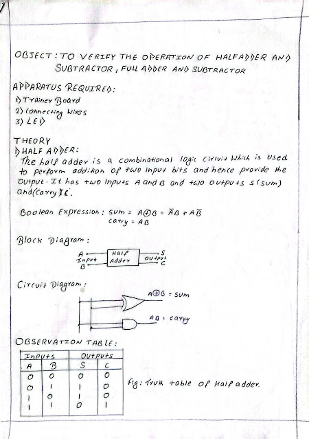

Comments
Post a Comment